Spatio-temporal prediction package


Project description
stpredict package


stpredict is designed to apply forecasting methods on spatio-temporal data to predict the values of a target variable in the future time points based on the historical values of the features. The main stages of the modeling process are implemented in this package including:
- Data preprocessing
- Data partitioning
- Feature selection
- Model selection
- Model evaluation
- Prediction
Installation
pip install stpredict
When package is installed, it's functions can be used to process the spatio-temporal data. stpredict provides a flexible data structure to receive a spatio-temporal data in functions. Input data of the preprocess module functions can be presented in two dataframes:
-
Temporal data: Temporal data includes the information of the variables that are time-varying and their values change over time. Temporal data must include columns:
- Spatial ids: ids of spatial units.
- Temporal ids: ids of temporal units, which may be included in integrated or non-integrated format. As an example, in Figure 1 temporal ids can be the date of the week last day (integrated), or the year and number of the week (non-integrated).
- Temporal covariates
- Target
-
Spatial data: Spatial data includes the information on variables which their values only depend on the spatial aspect of the problem. spatial data must includes following columns:
- Spatial ids: The id of the units in the finest spatial scale of input data must be included in the spatial data. As it is shown in Figure 1, ids of secondary spatial scale can be included in the spatial and temporal data tables or be received in a separate input (i.e. spatial scale table).
- Spatial covariates

Fig.1 Input data tables
The complete list of functions can be find in documentation. The main functions are as follows:
1. preprocess_data
preprocess.preprocess_data(data, forecast_horizon, history_length = 1,
			   column_identifier = None, spatial_scale_table = None,
			   spatial_scale_level = 1, temporal_scale_level = 1,
			   target_mode = 'normal', imputation = True,
			   aggregation_mode = 'mean', augmentation = False,
			   futuristic_covariates = None, future_data_table = None,
			   save_address = None, verbose = 0)
Perform all steps of preprocessing including:
- Imputation: Imputation of missing values are implemented by taking advantage of same temporal pattern in different spatial units, and the missing values of a spatial unit at given temporal unit is imputed using the values of the spatial units with the most similar temporal pattern. As an example, if precipitation of a city is missing for a given year, it is imputed using the average precipitation of cities having the most similar precipitation trend over years. If some spatial units have only missing values, they will be removed from the data (Figure 2).

Fig.2 Imputation of missing values in temporal data
- Scale modification: Changing the temporal(spatial) scale of data by calculation of sum or average values of units in smaller scale. An example is shown in Figure 3 where the variable values of the US counties are aggregated to obtain a value for each state.
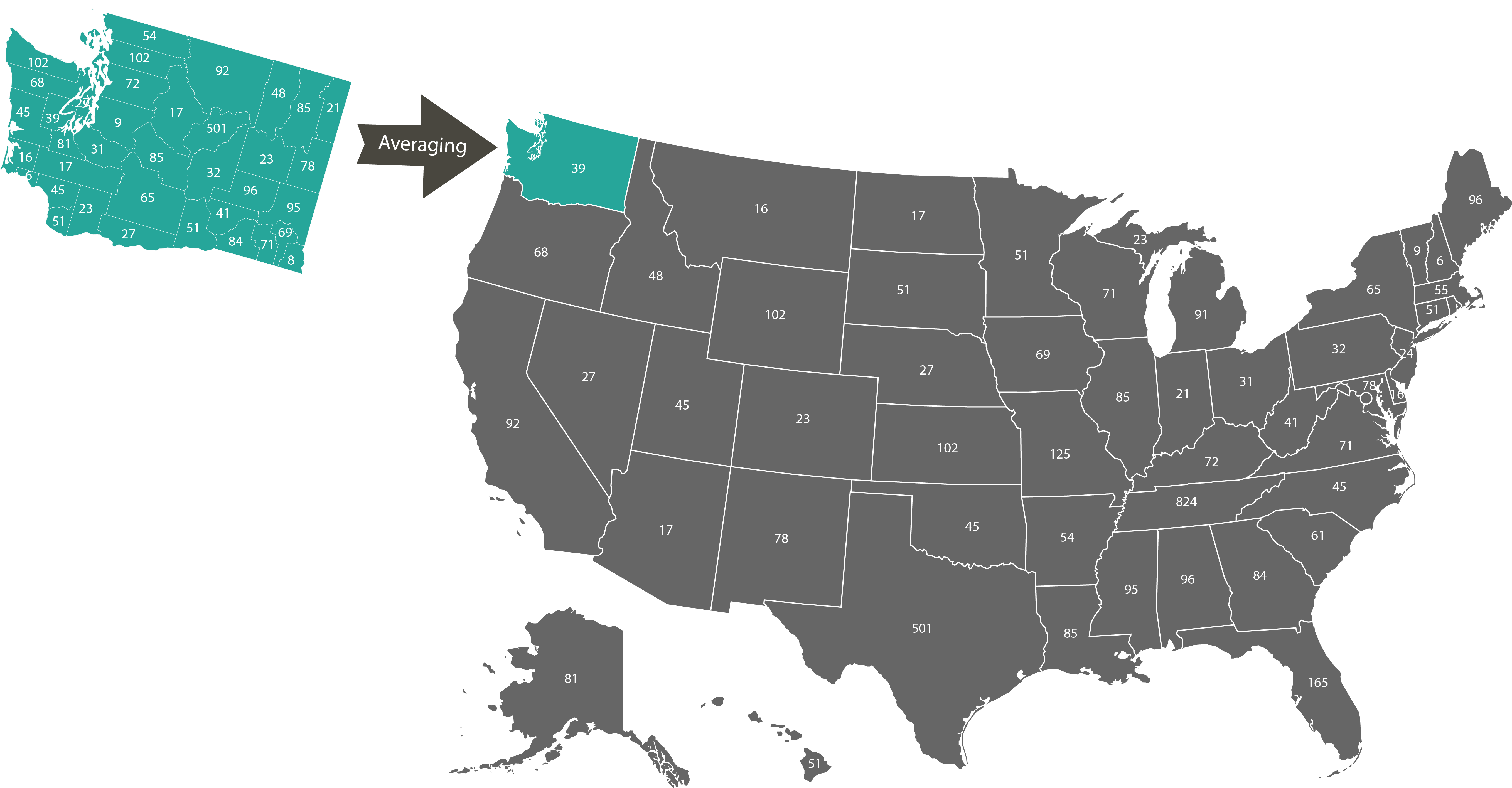
Fig.3 Spatial scale transform
Users can also use augmentation argument to augment data when using bigger temporal scales and avoid data volume decrease. For this purpose, in the process of temporal scale transformation, instead of taking the average of smaller scale units’ values to get the bigger scale unit value, the moving average method is used. Figures 4 and 5 represents temporal scale transformation (day->week) with and without augmentation.
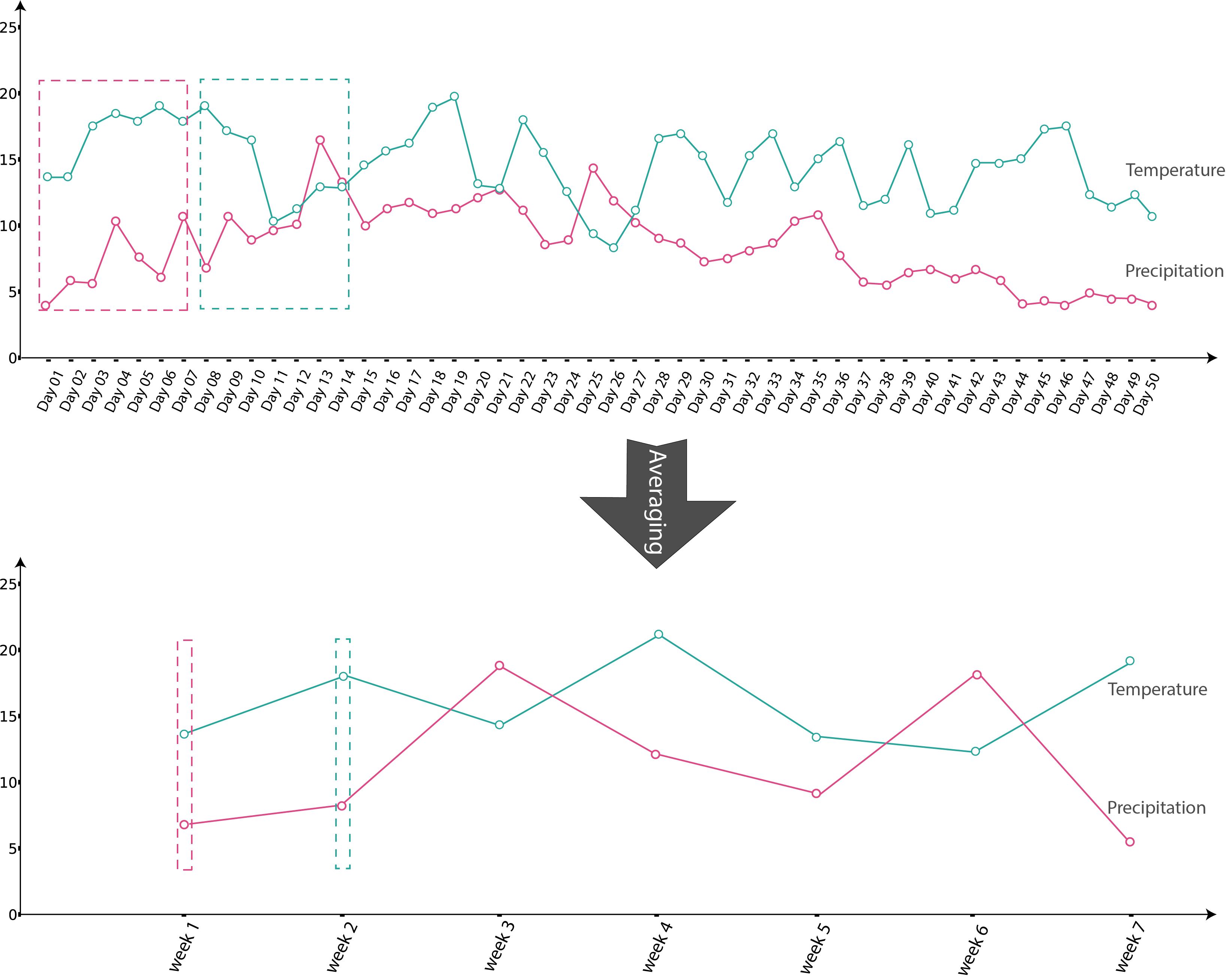
Fig.4 Temporal scale transform without augmentation
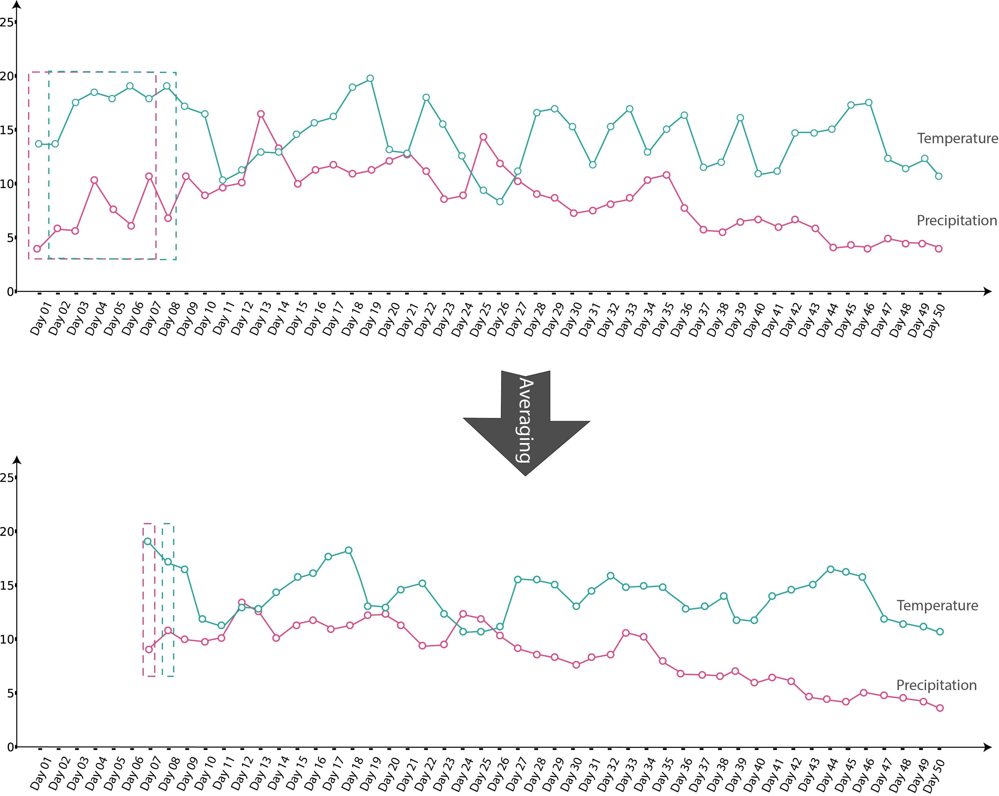
Fig.5 Temporal scale transform with augmentation
-
Target modification: modifing the target variable values to the cumulative or moving average values.
-
Historical data: Transforming input data to the historical format that can be used to train the models for prediction of target variable based on past values of covariates. The final set of features consists of spatial covariates, temporal covariates at current temporal unit (t) and historical values of these covariates at h-1 previous temporal units (t-1 , t-2 , … , t-h+1). The target of the output data frame is the values of the target variable at the temporal unit t+r, where h and r denote the user specified history length and forecast horizon (Figure 6) . In addition, if the user prefers to output data frame(s) include the values of some covariates in the future temporal units as features, the name of these covariates could be specified using the
futuristic_covariatesargument.

Fig.6 Historical data
Each of this steps are also provided in separate functions as follows.
# Imputation
preprocess.impute(data, column_identifier = None, verbose = 0)

# Change temporal scale
preprocess.temporal_scale_transform(data, column_identifier = None,
				    temporal_scale_level = 2, augmentation = False,
				    verbose = 0)

# Change spatial scale
preprocess.spatial_scale_transform(data, data_type, spatial_scale_table = None,
				   spatial_scale_level = 2, aggregation_mode = 'mean',
				   column_identifier = None, verbose = 0)

# Modify target variable values to cumulative, moving average, or differential values
preprocess.target_modification(data, target_mode, column_identifier = None, verbose = 0)

# Make historical data
preprocess.make_historical_data(data, forecast_horizon, history_length = 1,
				column_identifier = None, futuristic_covariates = None,
				future_data_table = None, step = 1, verbose = 0)
2. predict
predict.predict(data, forecast_horizon,  feature_sets = {'covariate':'mRMR'},
		forced_covariates = [], models = ['knn'],  mixed_models = ['knn'],
		model_type = 'regression', test_type = 'whole-as-one',
		splitting_type = 'training-validation',  instance_testing_size = 0.2,
		instance_validation_size = 0.3, instance_random_partitioning = False,
		fold_total_number = 5, feature_scaler = None, target_scaler = None,
		performance_benchmark = 'MAPE',  performance_measure = ['MAPE'],
		performance_mode = 'normal', scenario = ‘current’,
		validation_performance_report = True, testing_performance_report = True,
		save_predictions = True, save_ranked_features = True,
		plot_predictions = False, verbose = 0)
Split data to the training, validation and testing sets. Selecting the model, featureset, and length of history to optimize the prediction performance and based on the model performance on validation set. Report the performance of the best model on testing set and predict the future values of the target variable.
The predict function is implemented by calling smaller functions, each of which executes part of the modeling process. These functions are as follows.
# Data splitting
predict.split_data(data, splitting_type = 'instance', instance_testing_size = None,
               instance_validation_size = None, instance_random_partitioning = False,
               fold_total_number = None, fold_number = None, forecast_horizon = 1,
               granularity = 1, verbose = 0)

# Select the best model, history length, and feature set
predict.train_validate(data, feature_sets, forced_covariates=[],
		instance_validation_size=0.3, instance_testing_size=0, fold_total_number=5,
		instance_random_partitioning=False, forecast_horizon=1, models=['knn'],
		mixed_models=None, model_type='regression',
		splitting_type='training-validation', performance_measures=None,
                performance_benchmark=None, performance_mode='normal', feature_scaler=None,
                target_scaler=None, labels=None, performance_report=True,
		save_predictions=True, verbose=0)

# Slice the dataframe and return a dataframe including only the selected features
predict.select_features(data, ordered_covariates_or_features)

# Calculate predictive performance
predict.performance(true_values, predicted_values, performance_measures=['MAPE'],
		trivial_values=[], model_type='regression', num_params=1,
		labels=None)

# Train the best model and report the performance on test set
predict.train_test(data, instance_testing_size, forecast_horizon, feature_or_covariate_set,
               history_length, model='knn', base_models=None, model_type='regression',
               model_parameters=None, feature_scaler='logarithmic',
	       target_scaler='logarithmic', labels=None, performance_measures=['MAPE'],
	       performance_mode='normal', performance_report=True, save_predictions=True,
	       verbose=0)

# Predict future values of the target variable
predict.predict_future(data, future_data, forecast_horizon, feature_or_covariate_set,
		       model = 'knn', base_models = [], model_type = 'regression',
		       model_parameters = None, feature_scaler = None, target_scaler = None,
		       labels = None, scenario  = 'current', save_predictions = True,
		       verbose = 0)
Figure 7 and 8 represents the whole process of prediction which can be performed in two different ways with regards to the test_type argument.
- If
test_type = whole-as-one, the prediction for all the test samples is made with the best model, feature set and history length which are obtained based on the prediction results of an identical training and validation set. The training and validation sets in this mode are obtained by removing all the test instances from the data. - If
test_type = one-by-one, each test sample has an different training and validation sets which obtained by removing only this test sample, and all of its subsequent test samples from the data. Using this method, more samples is used for training the model.

Fig.7 prediction process with test_type = whole-as-one

Fig.8 prediction process with test_type = one-by-one
As can be seen in these figures, the first function call is train_validate where the best model, history length, and feature set is selected. The selected model then will be used to measure performance on testing set (train_test) and finaly predict the future values of the target variable (predict_future). Figure 9 represent the train_validate function with details.

Fig.9 Details of train_validate function
Data splitting in stpredict is performed with regards to the temporal dimension of the historical data (See split_data). Testing data is selected from the last available temporal units. As an example, splitting of the historical data with the test size 1, history length 3 and forecast horizon 3 is shown in Figure 10. Each block represents an instance and its arrow indicates the date of the target variable. One sample related to the last available temporal units is selected as test set. Since the goal is to predict the target variable values of the test set sample that is at the temporal unit ‘27/01/20’ and our forecast horizon is 3, we only can use the data available until temporal unit ‘24/01/20’ which has 3 temporal units distance up to ‘26/01/20’. Therefore with regards to the forecast horizon r, the number of r-1 samples which their target values occur in this time interval are removed from training data which is shown as a gap in the figure.
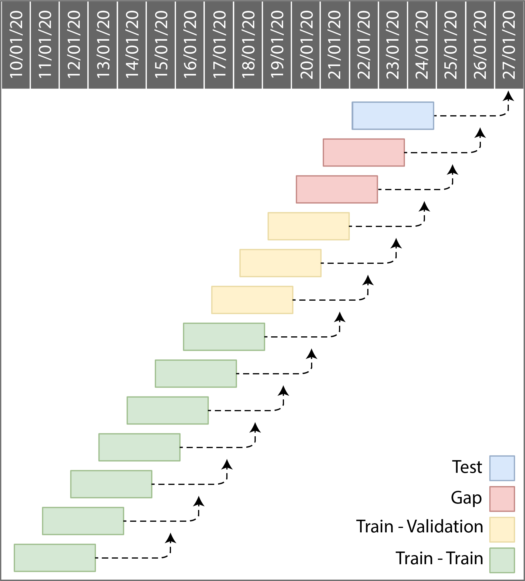
Fig.10 Temporal data splitting in stpredict
Some of the more important options in predict function are:
-
Feature selection mode: Using feature_sets argument user can select:
- The method of ranking which is used to rank the features(covariates) from the supported methods ‘correlation’, ‘mRMR’, and ‘variance’. If ‘correlation’, covariates(or features) are ranked based on their correlation with target variable. If ‘mRMR’ the ranking will be conducted based on mRMR method in which the correlation between the features themselves also affects the choice of rank. If ‘variance’ the variance-based sensitivity analysis method will be used in which covariates(features) are prioritized based on the fraction of target variable variance that can be attributed to their variance.
- To rank the covariates or all the features (covariates and their historical values).
The candid feature sets will be obtained by slicing the ranked list of covariates or features from the first item to item number n where n is varied from 1 to the total number of list items, and if items are covariates, the covariates in each resulting subset along with their corresponding historical values will form a candid feature set in the feature selection process.
-
Scenario: To determine the effect of future features on the target variable, users can set the
scenarioargument and check the predicted values of the target variable when the future values of futuristic features are set to min, max, mean or last observed value for these features.
In addition to these options predict function provided users with various options for data splitting, data scaling, performance evaluation, and the ability of visualize predictions.
3. stpredict
stpredict implements all steps of preprocessing and prediction in one function.
stpredict(data, forecast_horizon, history_length = 1, column_identifier = None,
	  feature_sets = {'covariate': 'mRMR'}, models = ['knn'], model_type = 'regression',
	  test_type = 'whole-as-one', mixed_models = [], performance_benchmark = 'MAPE',
	  performance_measures = ['MAPE'], performance_mode = 'normal',
	  splitting_type = 'training-validation', instance_testing_size = 0.2,
	  instance_validation_size = 0.3, instance_random_partitioning = False,
	  fold_total_number = 5, imputation = True, target_mode = 'normal',
	  feature_scaler = None, target_scaler = None, forced_covariates = [],
	  futuristic_covariates = None, scenario = 'current', future_data_table = None,
	  temporal_scale_level = 1, spatial_scale_level = 1, spatial_scale_table = None,
	  aggregation_mode = 'mean', augmentation = False,
	  validation_performance_report = True, testing_performance_report = True,
	  save_predictions = True, save_ranked_features = True, plot_predictions = False,
	  verbose = 0)
Acknowledgements
We would thanks Dr. Zeinab Maleki and Dr. Pouria Ramazi for supervising this project. We also like to acknowledge the assistance of Nasrin Rafiei for development of the package.
Release history Release notifications | RSS feed


Download files
Download the file for your platform. If you're not sure which to choose, learn more about installing packages.
Source Distribution
Built Distribution
Filter files by name, interpreter, ABI, and platform.
If you're not sure about the file name format, learn more about wheel file names.
Copy a direct link to the current filters
File details
Details for the file stpredict-0.0.6.tar.gz.
File metadata
- Download URL: stpredict-0.0.6.tar.gz
- Upload date:
- Size: 84.2 kB
- Tags: Source
- Uploaded using Trusted Publishing? No
- Uploaded via: twine/3.4.2 importlib_metadata/4.6.1 pkginfo/1.7.1 requests/2.25.1 requests-toolbelt/0.9.1 tqdm/4.60.0 CPython/3.9.5
File hashes
| Algorithm | Hash digest | |
|---|---|---|
| SHA256 |
d93d5dd860ef278176f8959a799c8b3a82c4d0aaaa98594c999f7986c8af368d
|
|
| MD5 |
315959fcb99ffecf02479973308da7ec
|
|
| BLAKE2b-256 |
bce9bce76cc4b4fabfda05c6cc815fe7cfba87c568c50f64d79fe2f58302a150
|
File details
Details for the file stpredict-0.0.6-py3-none-any.whl.
File metadata
- Download URL: stpredict-0.0.6-py3-none-any.whl
- Upload date:
- Size: 91.3 kB
- Tags: Python 3
- Uploaded using Trusted Publishing? No
- Uploaded via: twine/3.4.2 importlib_metadata/4.6.1 pkginfo/1.7.1 requests/2.25.1 requests-toolbelt/0.9.1 tqdm/4.60.0 CPython/3.9.5
File hashes
| Algorithm | Hash digest | |
|---|---|---|
| SHA256 |
548f7619a5d2a685258a517601a64b4e63e1988d1ea56b4a5bbc356442ad9028
|
|
| MD5 |
28dcefa43952eba297c2585ae244ad0e
|
|
| BLAKE2b-256 |
dd2b6600416e062c2ee13cb5144dd70e1581c0c4d04b1aa4e498862cf04fdd2a
|


