A statistical test and plotting function for time-series data in general,

Project description
Time Series Test
Statistical testing and plotting functions for time-series data in general, and data from cognitive-pupillometry and electroencephalography (EEG) experiments in particular. Based on linear mixed effects modeling (or regular multiple linear regression), crossvalidation, and cluster-based permutation testing.
Sebastiaan Mathôt (@smathot)
Copyright 2021 - 2024


Contents
Citation
Mathôt, S., & Vilotijević, A. (2022). Methods in cognitive pupillometry: design, preprocessing, and analysis. Behavior Research Methods. https://doi.org/10.1101/2022.02.23.481628
About
This library provides two main functions for statistical testing of time-series data: lmer_crossvalidation_test() and lmer_permutation_test(). For a detailed description, see the manuscript above, but below a short introduction to both functions with their respective advantages and disadavantages.
When to use crossvalidation?
In general terms, lmer_crossvalidation_test() implements a statistical test for a specific-yet-common question when analyzing time-series data:
Do one or more independent variables affect a continuously recorded dependent variable (a 'time series') at any point in time?
When to use this test:
- For time series consisting of only a single component, that is, when each independent variable has only a single effect on the time series. An example of this is the effect of stimulus intensity on pupil size, when presenting light flashes of different intensities.
- When you do not know a priori which time points to test.
When not to use this test:
- For time series that contain multiple components, that is, when each independent variable affects the time series in multiple ways that change over time. An example of this is the effect of visual attention on lateralized EEG recordings, where different EEG components emerge at different points in time.
- When you know a priori which time points to test.
More specifically, lmer_crossvalidation_test() locates and statistically tests effects in time-series data. It does so by using crossvalidation to identify time points to test, and then using a linear mixed effects model to actually perform the statistical test. More specifically, the data is subdivided in a number of subsets (by default 4). It takes one of the subsets (the test set) out of the full dataset, and conducts a linear mixed effects model on each sample of the remaining data (the training set). The sample with the highest absolute z value in the training set is used as the sample-to-be-tested for the test set. This procedure is repeated for all subsets of the data, and for all fixed effects in the model. Finally, a single linear mixed effects model is conducted for each fixed effects on the samples that were thus identified.
This packages also provides a function (plot()) to visualize time-series data to visually annotate the results of lmer_crossvalidation_test().
When to use lmer_permutation_test()?
lmer_permutation_test() implements a fairly standard cluster-based permutation test, which differs from most other implementations in that it relies on linear mixed-effects modeling to calculate the test statistics. Therefore, this function tends to be extremely computationally intensive, but should also be more sensitive than cluster-based permutation tests that are based on average data. Its main advantage as compared to lmer_crossvalidation_test() is that it is also valid for data with multiple components, such as event-related potentials (ERPs).
Can the tests also be based on regular multiple regression (instead of linear mixed effects modeling)?
Yes. If you pass groups=None to any of the functions, the analysis will be based on a regular multiple linear regression instead of linear mixed effects modeling.
Installation
pip install time_series_test
Dependencies
Usage
We will use data from Zhou, Lorist, and Mathôt (2021). In brief, this is data from a visual-working-memory experiment in which participant memorized one or more colors (set size: 1, 2, 3 or 4) of two different types (color type: proto, nonproto) while pupil size was being recorded during a 3s retention interval.
This dataset contains the following columns:
pupil, which is is our dependent measure. It is a baseline-corrected pupil time series of 300 samples, recorded at 100 Hzsubject_nr, which we will use as a random effectset_size, which we will use as a fixed effectcolor_type, which we will use as a fixed effect
First, load the dataset:
from datamatrix import io
dm = io.readpickle('data/zhou_et_al_2021.pkl')
The plot() function provides a convenient way to plot pupil size over time as a function of one or two factors, in this case set size and color type:
import time_series_test as tst
from matplotlib import pyplot as plt

tst.plot(dm, dv='pupil', hue_factor='set_size', linestyle_factor='color_type',
         sampling_freq=100)
plt.savefig('img/signal-plot-1.png')
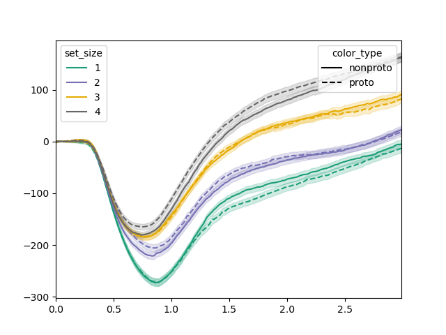
From this plot, we can tell that there appear to be effects in the 1500 to 2000 ms interval. To test this, we could perform a linear mixed effects model on this interval, which corresponds to samples 150 to 200.
The model below uses mean pupil size during the 150 - 200 sample range as dependent measure, set size and color type as fixed effects, and a random by-subject intercept. In the more familiar notation of the R package lme4, this corresponds to mean_pupil ~ set_size * color_type + (1 | subject_nr). (To use more complex random-effects structures, you can use the re_formula argument to mixedlm().)
from statsmodels.formula.api import mixedlm
from datamatrix import series as srs, NAN

dm.mean_pupil = srs.reduce(dm.pupil[:, 150:200])
dm_valid_data = dm.mean_pupil != NAN
model = mixedlm(formula='mean_pupil ~ set_size * color_type',
                data=dm_valid_data, groups='subject_nr').fit()
print(model.summary())
Output:
                    Mixed Linear Model Regression Results
=============================================================================
Model:                    MixedLM       Dependent Variable:       mean_pupil
No. Observations:         7300          Method:                   REML
No. Groups:               30            Scale:                    38610.3390
Min. group size:          235           Log-Likelihood:           -48952.3998
Max. group size:          248           Converged:                Yes
Mean group size:          243.3
-----------------------------------------------------------------------------
                              Coef.   Std.Err.   z    P>|z|  [0.025   0.975]
-----------------------------------------------------------------------------
Intercept                    -144.024   17.438 -8.259 0.000 -178.202 -109.846
color_type[T.proto]           -24.133   11.299 -2.136 0.033  -46.278   -1.987
set_size                       49.979    2.906 17.200 0.000   44.284   55.675
set_size:color_type[T.proto]   10.176    4.120  2.470 0.014    2.101   18.251
subject_nr Var               7217.423    9.882
=============================================================================
The model summary shows that, assuming an alpha level of .05, there are significant main effects of color type (z = -2.136, p = .033), set size (z = 17.2, p < .001), and a significant color-type by set-size interaction (z = 2.47, p = .014). However, we have selectively analyzed a sample range that we knew, based on a visual inspection of the data, to show these effects. This means that our analysis is circular: we have looked at the data to decide where to look! The find() function improves this by splitting the data into training and tests sets, as described under About, thus breaking the circularity.
results = tst.find(dm, 'pupil ~ set_size * color_type',
                   groups='subject_nr', winlen=5)
The return value of find() is a dict, where keys are effect labels and values are named tuples of the following:
model: a model as returned bymixedlm().fit()samples: asetwith the sample indices that were usedp: the p-value from the modelz: the z-value from the model
The summarize() function is a convenient way to get the results in a human-readable format.
print(tst.summarize(results))
Output:
Intercept was tested at samples {95} → z = -13.1098, p = 2.892e-39, converged = yes
color_type[T.proto] was tested at samples {160, 170, 175} → z = -2.0949, p = 0.03618, converged = yes
set_size was tested at samples {185, 210, 195, 255} → z = 16.2437, p = 2.475e-59, converged = yes
set_size:color_type[T.proto] was tested at samples {165, 175} → z = 2.5767, p = 0.009974, converged = yes
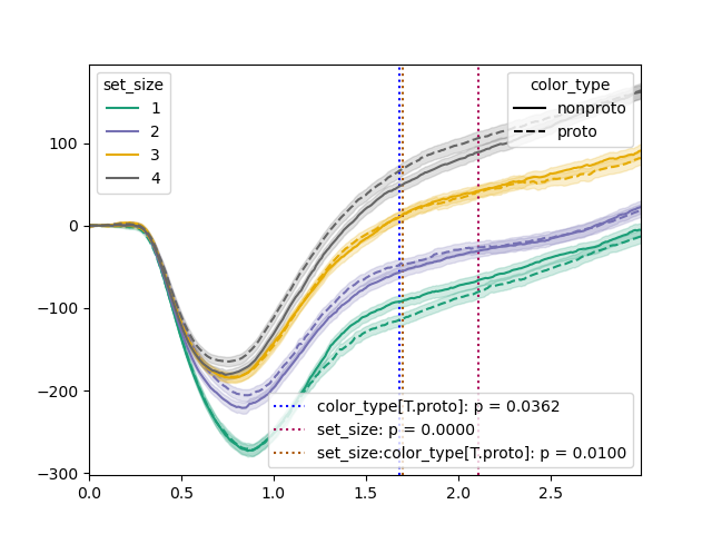
We can pass the results to plot() to visualize the results:
plt.clf()
tst.plot(dm, dv='pupil', hue_factor='set_size', linestyle_factor='color_type',
         results=results, sampling_freq=100)
plt.savefig('img/signal-plot-2.png')
Function reference
time_series_test.lmer_crossvalidation_test(dm, formula, groups, re_formula=None, winlen=1, split=4, split_method='interleaved', samples_fe=True, samples_re=True, localizer_re=False, fit_method=None, suppress_convergence_warnings=False, fit_kwargs=None, **kwargs)
Conducts a single linear mixed effects model to a time series, where the to-be-tested samples are determined through crossvalidation.
This function uses mixedlm() from the statsmodels package. See the
statsmodels documentation for a more detailed explanation of the
parameters.
Parameters
-
dm: DataMatrix
The dataset
-
formula: str
A formula that describes the dependent variable, which should be the name of a series column in
dm, and the fixed effects, which should be regular (non-series) columns. -
groups: str or None or list of str
The groups for the random effects, which should be regular (non-series) columns in
dm. IfNoneis specified, then all analyses are based on a regular multiple linear regression (instead of linear mixed effects model). -
re_formula: str or None
A formula that describes the random effects, which should be regular (non-series) columns in
dm. -
winlen: int, optional
The number of samples that should be analyzed together, i.e. a downsampling window to speed up the analysis.
-
split: int, optional
The number of splits that the analysis should be based on.
-
split_method: str, optional
If 'interleaved', the data is split in a regular interleaved fashion, such that the first row goes to the first subset, the second row to the second subset, etc. If 'random', the data is split randomly in subsets. Interleaved splitting is deterministic (i.e. it results in the same outcome each time), but random splitting is not.
-
samples_fe: bool, optional
Indicates whether sample indices are included as an additive factor to the fixed-effects formula. If all splits yielded the same sample index, this is ignored.
-
samples_re: bool, optional
Indicates whether sample indices are included as an additive factor to the random-effects formula. If all splits yielded the same sample index, this is ignored.
-
localizer_re: bool, optional
Indicates whether a random effects structure as specified using the
re_formulakeyword should also be used for the localizer models, or only for the final model. -
fit_kwargs: dict or None, optional
A
dictthat is passed as keyword arguments tomixedlm.fit(). For example, to specify the nm as the fitting method, specifyfit_kwargs={'fit': 'nm'}. -
fit_method: str, list of str, or None, optional
Deprecated. Use
fit_kwargsinstead. -
suppress_convergence_warnings: bool, optional
Installs a warning filter to suppress conververgence (and other) warnings.
-
**kwargs: dict, optional
Optional keywords to be passed to
mixedlm().
Returns
-
dict
A dict where keys are effect labels, and values are named tuples of
model,samples,p, andz.
time_series_test.lmer_permutation_test(dm, formula, groups, re_formula=None, winlen=1, suppress_convergence_warnings=False, fit_kwargs={}, iterations=1000, cluster_p_threshold=0.05, test_intercept=False, **kwargs)
Performs a cluster-based permutation test based on sample-by-sample linear-mixed-effects analyses. The permutation test identifies clusters based on p-value threshold and uses the absolute of the summed z-values of the clusters as test statistic.
If no clusters reach the threshold, the test is skipped right away. By
default the Intercept is ignored for this criterion, because the intercept
usually has significant clusters that we're not interested in. However, you
can change this using the test_intercept keyword.
Warning: This is generally an extremely time-consuming analysis because it requires thousands of lmers to be run.
See lmer_crossvalidation() for an explanation of the arguments.
Parameters
-
dm: DataMatrix
-
formula: str
-
groups: str
-
re_formula: str or None, optional
-
winlen: int, optional
-
suppress_convergence_warnings: bool, optional
-
fit_kwargs: dict, optional
-
iterations: int, optional
The number of permutations to run.
-
cluster_p_threshold: float or None, optional
The maximum p-value for a sample to be considered part of a cluster.
-
test_intercept: bool, optional
Indicates whether the intercept should be included when considering if there are any clusters, as described above.
-
**kwargs: dict, optional
Returns
-
dict
A dict with effects as keys and lists of clusters defined by (start, end, z-sum, hit proportion) tuples. The p-value is 1 - hit proportion.
time_series_test.lmer_series(dm, formula, winlen=1, fit_kwargs={}, **kwargs)
Performs a sample-by-sample linear-mixed-effects analysis. See
lmer_crossvalidation() for an explanation of the arguments.
Parameters
-
dm: DataMatrix
-
formula: str
-
winlen: int, optional
-
fit_kwargs: dict, optional
-
**kwargs: dict, optional
Returns
-
DataMatrix
A DataMatrix with one row per effect, including the intercept, and three series columns with the same depth as the dependent measure specified in the formula:
est: the slopep: the p valuez: the z valuese: the standard error
time_series_test.plot(dm, dv, hue_factor, results=None, linestyle_factor=None, hues=None, linestyles=None, alpha_level=0.05, annotate_intercept=False, annotation_hues=None, annotation_linestyle=':', legend_kwargs=None, annotation_legend_kwargs=None, x0=0, sampling_freq=1)
Visualizes a time series, where the signal is plotted as a function of
sample number on the x-axis. One fixed effect is indicated by the hue
(color) of the lines. An optional second fixed effect is indicated by the
linestyle. If the results parameter is used, significant effects are
annotated in the figure.
Parameters
-
dm: DataMatrix
The dataset
-
dv: str
The name of the dependent variable, which should be a series column in
dm. -
hue_factor: str
The name of a regular (non-series) column in
dmthat specifies the hue (color) of the lines. -
results: dict, optional
A
resultsdict as returned bylmer_crossvalidation(). -
linestyle_factor: str, optional
The name of a regular (non-series) column in
dmthat specifies the linestyle of the lines for a two-factor plot. -
hues: str, list, or None, optional
The name of a matplotlib colormap or a list of hues to be used as line colors for the hue factor.
-
linestyles: list or None, optional
A list of linestyles to be used for the second factor.
-
alpha_level: float, optional
The alpha level (maximum p value) to be used for annotating effects in the plot.
-
annotate_intercept: bool, optional
Specifies whether the intercept should also be annotated along with the fixed effects.
-
annotation_hues: str, list, or None, optional
The name of a matplotlib colormap or a list of hues to be used for the annotations if
resultsis provided. -
annotation_linestyle: str, optional
The linestyle for the annotations.
-
legend_kwargs: None or dict, optional
Optional keywords to be passed to
plt.legend()for the factor legend. -
annotation_legend_kwargs: None or dict, optional
Optional keywords to be passed to
plt.legend()for the annotation legend. -
x0: int, float
The starting value on the x-axis.
-
sampling_freq: int, float
The sampling frequency.
time_series_test.summarize(results, detailed=False)
Generates a string with a human-readable summary of a results dict as
returned by lmer_crossvalidation().
Parameters
-
results: dict
A
resultsdict as returned bylmer_crossvalidation(). -
detailed: bool, optional
Indicates whether model details should be included in the summary.
Returns
- str
License
time_series_test is licensed under the GNU General Public License
v3.
Release history Release notifications | RSS feed


Download files
Download the file for your platform. If you're not sure which to choose, learn more about installing packages.
Source Distribution
Built Distribution
Filter files by name, interpreter, ABI, and platform.
If you're not sure about the file name format, learn more about wheel file names.
Copy a direct link to the current filters
File details
Details for the file time_series_test-0.13.1.tar.gz.
File metadata
- Download URL: time_series_test-0.13.1.tar.gz
- Upload date:
- Size: 29.9 kB
- Tags: Source
- Uploaded using Trusted Publishing? No
- Uploaded via: twine/5.1.1 CPython/3.9.20
File hashes
| Algorithm | Hash digest | |
|---|---|---|
| SHA256 |
055c44b918852a07c20c55c7315b8c16e205febc3b4585803038dfb65b65778e
|
|
| MD5 |
57565a9ac3d698f53ba8dbb29209b79e
|
|
| BLAKE2b-256 |
1ceff2f90ba77cfa5f1770b1e5ec35670a9f7cc461202dd9858ea6a0361100f3
|
File details
Details for the file time_series_test-0.13.1-py3-none-any.whl.
File metadata
- Download URL: time_series_test-0.13.1-py3-none-any.whl
- Upload date:
- Size: 27.2 kB
- Tags: Python 3
- Uploaded using Trusted Publishing? No
- Uploaded via: twine/5.1.1 CPython/3.9.20
File hashes
| Algorithm | Hash digest | |
|---|---|---|
| SHA256 |
ee3ca961e046002eed251fd2d6f05ff2acb97264fe0e7499061695f86d14b7d2
|
|
| MD5 |
5a3f01275c1c18a1381bafc387d8cbf4
|
|
| BLAKE2b-256 |
c1633822a58c14d7a7541da366cff247ebfa20365ab5ec17ba4c4d690fce8ba6
|


