Library to run VI algorithms on Stan models.

Project description
vistan
vistan is a simple library to run variational inference algorithms on Stan models.
vistan uses autograd and PyStan under the hood, and aims to help you quickly run different variational methods from Advances in BBVI on Stan models.
Features
- Initialization: Laplace's method to initialize full-rank Gaussian
- Gradient Estimators: Total-gradient, STL, DReG, closed-form entropy
- Variational Families: Full-rank Gaussian, Diagonal Gaussian, RealNVP
- Objectives: ELBO, IW-ELBO
- IW-sampling: Posterior samples using importance weighting
Installation
pip install vistan
Usage
The typical usage of the package would have the following steps:
- Use default variational recipes as
vistan.recipe("meanfield"). There are various options:advi: Run our implementation of ADVI's PyStan.meanfield: Full-factorized Gaussia a.k.a meanfield VIfullrank: Use a full-rank Gaussian for better dependence between latent variablesflows: Use a RealNVP flow-based VImethod x: Use methods from the paper Advances in BBVI where x is one of[0, 1, 2, 3a, 3b, 4a, 4b, 4c, 4d]
- Create an algorithm as
algo=vistan.algorithm(). Some most frequent arguments:vi_family: This can be one of['gaussian', 'diagonal', 'rnvp'](Default:gaussian)max_iter: The maximum number of optimization iterations. (Default: 100)optimizer: This can beadamoradvi. (Default:adam)grad_estimator: What gradient estimator to use. Can beTotal-gradient,STL,DReG, orclosed-form-entropy. (Default:DReG)M_iw_train: The number of importance samples. Use 1 for standard variational inference or more for importance-weighted variational inference. (Default: 1)per_iter_sample_budget: The total number of evaluations to use in each iteration. (Default: 100)
- Get an approximate posterior as
posterior=algo(code, data). This runs the algorithm on Stan model given by the stringcodewith observations given by thedata. - Draw samples from the approximate posterior as
samples=posterior.sample(100). You can also draw samples using importance weighting asposterior.sample(100, M_iw_sample=10). Further, you can evaluate the log-probability of the posterior asposterior.log_prob(latents).
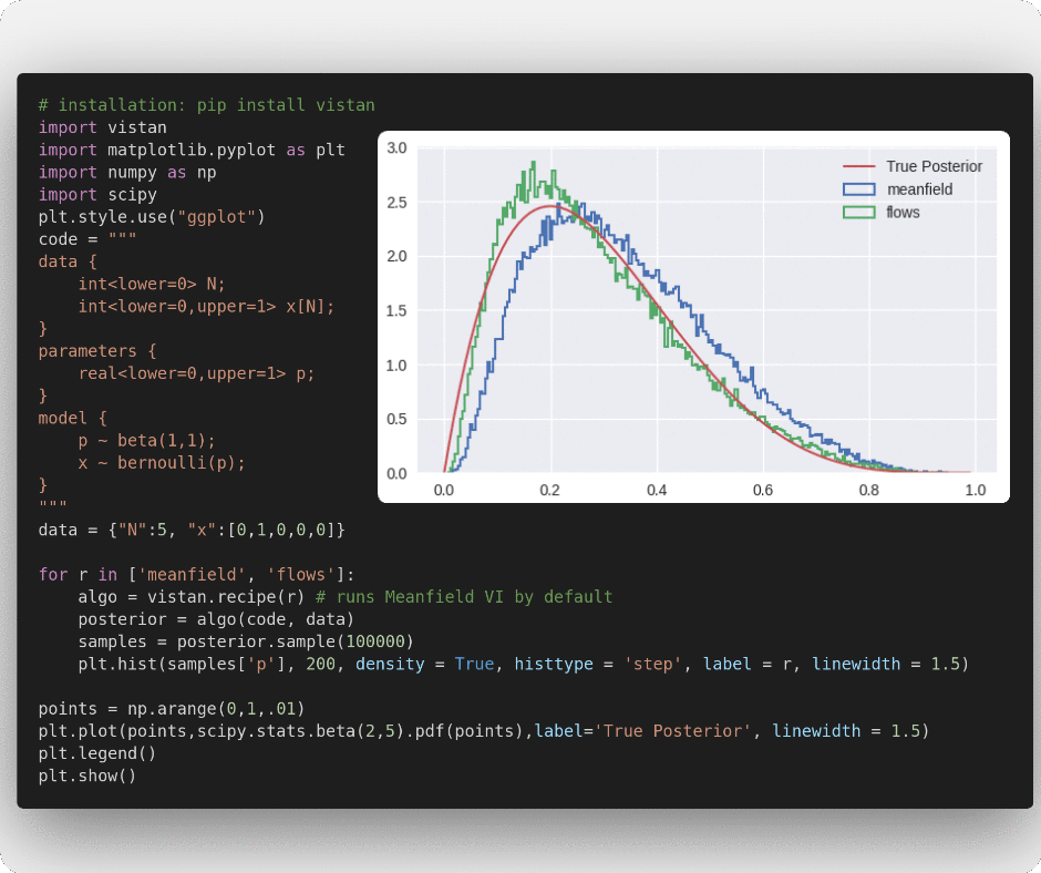
Recipes
Meanfield Gaussian
We provide some default VI algorithm choices which can accessed using vistan.recipe
import vistan
import matplotlib.pyplot as plt
import numpy as np
import scipy
code = """
data {
    int<lower=0> N;
    int<lower=0,upper=1> x[N];
}
parameters {
    real<lower=0,upper=1> p;
}
model {
    p ~ beta(1,1);
    x ~ bernoulli(p);
}
"""
data = {"N":5, "x":[0,1,0,0,0]}
algo = vistan.recipe() # runs Meanfield VI by default
posterior = algo(code, data)
samples = posterior.sample(100000)

points = np.arange(0,1,.01)
plt.hist(samples['p'], 200, density = True, histtype = 'step')
plt.plot(points,scipy.stats.beta(2,5).pdf(points),label='True Posterior')
plt.legend()
plt.show()
Full-rank Gaussian
algo = vistan.recipe("fullrank")
posterior = algo(code, data)
samples = posterior.sample(100000)

points = np.arange(0, 1, .01)
plt.hist(samples['p'], 200, density=True, histtype='step')
plt.plot(points, scipy.stats.beta(2, 5).pdf(points), label='True Posterior')
plt.legend()
plt.show()
Flow-based VI
algo = vistan.recipe("flows")
posterior = algo(code, data)
samples = posterior.sample(100000)

points = np.arange(0, 1, .01)
plt.hist(samples['p'], 200, density=True, histtype='step')
plt.plot(points, scipy.stats.beta(2, 5).pdf(points), label='True Posterior')
plt.legend()
plt.show()
ADVI
Our implementation of PyStan's ADVI.
algo = vistan.recipe("advi")
posterior = algo(code, data)
samples = posterior.sample(100000)

points = np.arange(0, 1, .01)
plt.hist(samples['p'], 200, density=True, histtype='step')
plt.plot(points, scipy.stats.beta(2, 5).pdf(points), label='True Posterior')
plt.legend()
plt.show()
Methods from Advances in BBVI
Our implementation of different variational methods from the paper.
# Try method 0, 1, 2, 3a, 3b, 4a, 4b, 4c, 4d
algo = vistan.recipe("method 4d")
posterior = algo(code, data)
samples = posterior.sample(100000)

points = np.arange(0, 1, .01)
plt.hist(samples['p'], 200, density=True, histtype='step')
plt.plot(points, scipy.stats.beta(2, 5).pdf(points), label='True Posterior')
plt.legend()
plt.show()
Custom algorithms
You can also specify custom VI algorithms to work with your Stan models using vistan.algorithm. Please, see the documentation of vistan.algorithm for a complete list of supported arguments.
algo = vistan.algorithm(
                M_iw_train=2,
                grad_estimator="DReG",
                vi_family="gaussian",
                per_iter_sample_budget=10,
                max_iters=100)
posterior = algo(code, data)
samples = posterior.sample(100000)

points = np.arange(0, 1, .01)
plt.hist(samples['p'], 200, density=True, histtype='step')
plt.plot(points, scipy.stats.beta(2, 5).pdf(points), label='True Posterior')
plt.legend()
plt.show()
IW-sampling
We provide support to use IW-sampling at inference time; this importance weights M_iw_sample candidate samples and picks one (see Advances in BBVI for more information.) IW-sampling is a post-hoc step and can be used with almost any variational scheme.
samples = posterior.sample(100000, M_iw_sample=10)

points = np.arange(0, 1, .01)
plt.hist(samples['p'], 200, density=True, histtype='step')
plt.plot(points, scipy.stats.beta(2, 5).pdf(points), label='True Posterior')
plt.legend()
plt.show()
Initialization
We provide support to use Laplace's method to initialize the parameters for Gaussian VI.
algo = vistan.algorithm(vi_family='gaussian', LI=True)
posterior = algo(code, data)
samples = posterior.sample(100000)

points = np.arange(0, 1, .01)
plt.hist(samples['p'], 200, density=True, histtype='step')
plt.plot(points, scipy.stats.beta(2, 5).pdf(points), label='True Posterior')
plt.legend()
plt.show()
Building your own inference algorithms
We provide access to the model.log_prob function we use internally for optimization. This allows you to evaluate the log density in the unconstrained space for your Stan model. Also, this function is differentiable in autograd.
log_prob = posterior.model.log_prob
Limitations
- We currently only support inference on all latent parameters in the model
- No support for data sub-sampling.
Release history Release notifications | RSS feed


Download files
Download the file for your platform. If you're not sure which to choose, learn more about installing packages.
Source Distribution
Built Distribution
Filter files by name, interpreter, ABI, and platform.
If you're not sure about the file name format, learn more about wheel file names.
Copy a direct link to the current filters
File details
Details for the file vistan-0.0.0.5.1.tar.gz.
File metadata
- Download URL: vistan-0.0.0.5.1.tar.gz
- Upload date:
- Size: 24.9 kB
- Tags: Source
- Uploaded using Trusted Publishing? No
- Uploaded via: twine/3.2.0 pkginfo/1.6.1 requests/2.25.0 setuptools/50.3.2.post20201201 requests-toolbelt/0.9.1 tqdm/4.54.1 CPython/3.9.0
File hashes
| Algorithm | Hash digest | |
|---|---|---|
| SHA256 |
d038f5604c023113130f72656018b5d4bc2edd6f4963bfd728646bdef8931fc6
|
|
| MD5 |
7b27a11c39b73aaa30ebdaeaea008bf1
|
|
| BLAKE2b-256 |
bf9c3d4f947d6f88db646e8b9217a9e13b099c2138e25b1bf4775c616431c2a1
|
File details
Details for the file vistan-0.0.0.5.1-py3-none-any.whl.
File metadata
- Download URL: vistan-0.0.0.5.1-py3-none-any.whl
- Upload date:
- Size: 42.0 kB
- Tags: Python 3
- Uploaded using Trusted Publishing? No
- Uploaded via: twine/3.2.0 pkginfo/1.6.1 requests/2.25.0 setuptools/50.3.2.post20201201 requests-toolbelt/0.9.1 tqdm/4.54.1 CPython/3.9.0
File hashes
| Algorithm | Hash digest | |
|---|---|---|
| SHA256 |
38a6eb365351a6dfe8fc5b049d8c3e056bb964399af087c5a26301813216d8fb
|
|
| MD5 |
4a4bea7f5d852fd230f9dfec03419085
|
|
| BLAKE2b-256 |
03422d3c2124340742d2a2f26e82e0497bd2095454c3f62dec7fc78f8e23a928
|


