
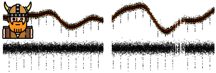





Wōtan...
...offers free and open source algorithms to automagically remove trends from time-series data.
In Germanic mythology, Odin (/ˈoːðinː/ Old High German: Wōtan) is a widely revered god. He gave one of his eyes to Mimir in return for wisdom. Thus, in order to achieve a goal, one sometimes has to turn a blind eye. In Richard Wagner's "Der Ring des Nibelungen", Wotan is the King of the Gods (god of light, air, and wind) and a bass-baritone. According to Wagner, he is the "pinnacle of intelligence".
What's new in 2.0
- Bugfixes: 31 bugs fixed (#70–#100), see BUGLOG.md. Highlights: the slider windows now include their last sample, masks work with any flux value, robust clipping is two-sided,
lowessuses a window in time units,cosine/cofiamwork for any time offset,psplineandrsplineconverge properly, and NaN/inf, unsorted time and invalid arguments are handled (with warnings instead of silent NaN trends). - Performance: all commonly used methods are faster, most of them by an order of magnitude (table below). The time-windowed sliders keep a sorted sliding window,
meanuses running sums, and sliders andlowessrun in parallel on all CPU cores;hsplinefits a sparse B-spline design matrix. Best case: themeandetrends ~32 million data points per second, thebiweight~2.3 million (1.x: ~19,000, 120x faster). Results agree with 1.x to 1e-6 (or 1e-3 of the noise, if larger), exceptcosineandcofiam, whose least-squares solution was made numerically stable (changes of up to ~1e-4). - Test coverage: a pytest suite of 563 tests covers all detrending methods, the API, edge cases, a regression test for every fixed bug, checks against independent reference implementations, and the trends of a real Kepler light curve against stored references. Run it with
pytest tests.
Speed: millions of data points per second
window_length=0.5 d, default parameters, 2 CPU cores (the parallel methods scale with the number of cores). Kepler-10: all 15 long-cadence quarters, 52k points (~25 points per window). White noise: 2-min cadence, no gaps, N points (~360 points per window). Reproduce with python benchmarks/bench.py --method <name>; details in benchmarks/RESULTS.md.
| Method | Kepler-10, 2.0 | Kepler-10, 1.x | White noise, 2.0 | White noise, 1.x | N (white) | Speed-up (geomean) |
|---|---|---|---|---|---|---|
mean |
34 | 2.5 | 32 | 1.1 | 1M | 19x |
median |
11 | 0.94 | 6.7 | 0.14 | 1M | 21x |
biweight |
5.0 | 0.12 | 2.3 | 0.019 | 1M | 60x |
hspline |
0.22 | 0.041 | 0.44 | 0.0082 | 100k | 14x |
rspline |
0.34 | 0.17 | 0.36 | 0.13 | 1M | 2.3x |
lowess |
0.33 | 0.037 | 0.18 | 0.020 | 100k | 9.1x |
cosine |
0.11 | 0.10 | 0.030 | 0.029 | 100k | 1.1x |
cofiam |
0.037 | 0.050 | 2.5 | 1.7 | 100k | 1.6x |
pspline |
– | – | 0.00076 | 0.00052 | 10k | 1.3x |
cofiam stops after a few harmonics on white noise, hence its high rate there; on Kepler-10 the numerically stable solution selects more harmonics than 1.x and is slower. pspline takes ~200 s for the Kepler-10 light curve and was benchmarked on its longest segment and 10k points only.
Example usage
from wotan import flatten
flatten_lc, trend_lc = flatten(time, flux, window_length=0.5, method='biweight', return_trend=True)
For more details, have a look at the interactive playground, the documentation. We also have examples and tutorials available, such as the 📑Example: Basic wotan functionality
Available detrending algorithms
-
Time-windowed sliders with location estimates: (📑Example: Comparison of sliders)
biweightRobust M-estimator using Tukey's biweight (📑Example)huberRobust M-estimator from Huber (1981) (iterative)huber_psiRobust M-estimator based on Huber's ψ (one-step)hampelRobust M-estimator based on Hampel (1972), 3-part descending, known as (a,b,c), 17A, 25AandrewsinewaveRobust M-estimator using Andrew's sine wavewelschRobust M-estimator from Welsch-LeclercramsayRobust M-estimator from Ramsay (1977), known as Ramsay's EatauRobust τ estimator from Yohai & Zamar (1986)hodgesRank-based robust R-estimator Hodges-Lehmann-SenmedianThe most robust (but least efficient)medfiltA cadence-based median filter (not time-windowed) for comparisonmeanThe least robust (but most efficient for white noise)trim_meanTrimmed mean (outliers are removed)winsorizeTrimmed mean (outliers are winsorized to a specified percentile)hampelfiltTrimmed mean (outliers are replaced with the median)
-
Splines: (📑Example)
rsplineSpline with iterative sigma-clippinghsplineSpline with a robust Huber estimator (Huber 1981)psplinePenalized spline to automatically select the knot distance (Eilers 1996), with iterative sigma-clipping
-
Polynomials and sines: (📑Example)
cofiamCosine Filtering with Autocorrelation Minimization (Kipping et al. 2013)cosineSum of sines and cosines, with option for iterative sigma-clippingsavgolSliding segments are fit with polynomials (Savitzky & Golay 1964), cadence-based
-
Regressions: (📑Example)
lowessLocally weighted scatterplot smoothing (Cleveland 1979)supersmootherFriedman's (1984) Super-Smoother, a local linear regression with adaptive bandwidth
Fitting a model that is a sum of Gaussian bases: (📑Example)
ridgeRidge regression (L2 loss, Tikhonov regularization)lassoLASSO regression (L1 loss, Least Absolute Shrinkage Selector Operator, Tibshirani (1996))elasticnetLinear regression model with 50% L1 and 50% L2 norm regularization
-
gpGaussian Processes offering: (📑Example: GP Standard vs. robust)squared_expSquared-exponential kernel, with option for iterative sigma-clippingmaternMatern 3/2 kernel, with option for iterative sigma-clippingperiodicPeriodic kernel informed by a user-specified period (📑Example)periodic_autoPeriodic kernel informed by a Lomb-Scargle periodogram pre-search
Available features
window_lengthThe length of the filter window in units oftime(usually days).break_toleranceIf there are large gaps in time, especially with corresponding flux level offsets, the detrending is much improved when splitting the data into several sub-lightcurves and applying the filter to each individually. Comes with an empirical default and is fully adjustable.edge_cutoffTrends near edges are less robust. Depending on the data, it may be beneficial to remove edges.cvalTuning parameter for the robust estimators (see documentation)return_trendIfTrue, the method will return a tuple of two elements (flattened_flux,trend_flux) wheretrend_fluxis the removed trend. Otherwise, it will only returnflattened_flux.transit_maskMask known transits during detrending (📑Example)
What method to choose?
It depends on your data and what you like to achieve (relevant xkcd). If possible, try it out! Use wotan with a selection of methods, iterate over their parameter space, and choose what gives the best results for your research.
If that is too much effort, you should first examine your data.
- Is it mostly white (Gaussian) noise? Use a time-windowed sliding mean. This is the most efficient method for white noise.
- With prominent outliers (such as transits or flares), use a robust time-windowed method such as the
biweight. This is usually superior to themedianor trimmed methods. - Are there (semi-) periodic trends? In addition to a time-windowed biweight, try a spline-based method. Experimenting with periodic GPs is worthwhile.
Installation
To install the released version, type
$ pip install wotan
which automatically installs numpy, numba and scipy if not present. Depending on the algorithm, additional dependencies exist:
huber,ramsay, andhampeldepend onstatsmodelshsplineandgpdepend onscikit-learnpsplinedepends onpygamsupersmootherdepends onsupersmoother
To install all additional dependencies, type $ pip install statsmodels scikit-learn supersmoother pygam.
For development: pip install -r tests/requirements-test.txt, then pytest runs the test suite (tests/README.md) and python benchmarks/bench.py --method biweight the benchmark (benchmarks/README.md). Note that numba's cache (*.nbi, *.nbc in __pycache__) does not track changes across files: after editing a compiled function that another one calls, delete the cache (find wotan -name "*.nb?" -delete), or the caller keeps the old code. Installed releases are not affected.
Originality
As all scientific work, wōtan is standing on the shoulders of giants. Particularly, many detrending methods are wrapped from existing packages. Original contributions include:
- A time-windowed detrending master module with edge treatments and segmentation options
- Robust location estimates using Newton-Raphson iteration to a precision threshold for Tukey's biweight, Andrew's sine wave, and the Welsch-Leclerc. This is probably a "first", which reduces jitter in the location estimate by ~10 ppm
- Robustified (iterative sigma-clipping) penalized splines for automatic knot distance determination and outlier resistance
- Robustified (iterative sigma-clipping) Gaussian processes
- GP with a periodic kernel informed by a Lomb-Scargle periodogram pre-search
- Bringing together many methods in one place in a common interface, with sensible defaults
- Providing documentation, tutorials, and a paper which compares and benchmarks the methods
Attribution
Please cite Hippke et al. (2019, AJ, 158, 143) if you find this code useful in your research. The BibTeX entry for the paper is:
@ARTICLE{2019AJ....158..143H,
       author = {{Hippke}, Michael and {David}, Trevor J. and {Mulders}, Gijs D. and
         {Heller}, Ren{\'e}},
        title = "{W{\={o}}tan: Comprehensive Time-series Detrending in Python}",
      journal = {\aj},
     keywords = {eclipses, methods: data analysis, methods: statistical, planetary systems, planets and satellites: detection, Astrophysics - Earth and Planetary Astrophysics, Astrophysics - Instrumentation and Methods for Astrophysics},
         year = "2019",
        month = "Oct",
       volume = {158},
       number = {4},
          eid = {143},
        pages = {143},
          doi = {10.3847/1538-3881/ab3984},
archivePrefix = {arXiv},
       eprint = {1906.00966},
 primaryClass = {astro-ph.EP},
       adsurl = {https://ui.adsabs.harvard.edu/abs/2019AJ....158..143H},
      adsnote = {Provided by the SAO/NASA Astrophysics Data System}
}
1 maintainer

Metadata
1 maintainer
Release files for wotan 2.0
For a detailed explanation of source distributions (sdists) and built distributions (wheels), please see the package formats documentation.
Source distribution (sdist)
| File | Size | Uploaded | |
|---|---|---|---|
| wotan-2.0.tar.gz | 69.2 kB | Details |
Built distribution (wheel)
| File | Interpreter | ABI | Platform | Reset |
|---|---|---|---|---|
| wotan-2.0-py3-none-any.whl | Python 3 | none | any | Details |
Total release size: 110.1 kB
Release files / wotan-2.0.tar.gz
| Download URL | wotan-2.0.tar.gz |
|---|---|
| Size | 69.2 kB |
| Tags | Source |
|
SHA-256 checksum How to use checksums |
6fcc5d5089f65e2259be1606583faf505cbb1c86d88809a21c51b83f73a60eb1
|
|
BLAKE2b-256 checksum How to use checksums |
c7fb753a294736ee337f5c97f2b4d6cfaaf20266d08c85c2fdda101841c6a705
|
| Upload date | |
|
Uploaded using Trusted Publishing? What is trusted publishing? |
No |
| Uploaded via |
twine/7.0.0 CPython/3.12.2
|
Release files / wotan-2.0-py3-none-any.whl
| Download URL | wotan-2.0-py3-none-any.whl |
|---|---|
| Size | 40.9 kB |
| Tags | Python 3 |
|
SHA-256 checksum How to use checksums |
13ed5b1b5f5d0dba9491e902c41a37268809b1a45b46547700a52f700870330f
|
|
BLAKE2b-256 checksum How to use checksums |
e4e2897a217eb7267985a22175f6379fd73309ed81166f367669a37a8a5a4aab
|
| Upload date | |
|
Uploaded using Trusted Publishing? What is trusted publishing? |
No |
| Uploaded via |
twine/7.0.0 CPython/3.12.2
|














