
 SpliPy
This repository contains the SpliPy packages. SpliPy is a pure python library for the creation, evaluation and manipulation of B-spline and NURBS geometries. It supports n-variate splines of any dimension, but emphasis is made on the use of curves, surfaces and volumes. The library is designed primarily for analysis use, and therefore allows fine-grained control over many aspects which is not possible to achieve with conventional CAD tools.
Features
SpliPy allows for the generation of parametric curves, surfaces and volumes in the form of non-uniform rational B-splines (NURBS). It supports traditional curve- and surface-fitting methods such as (but not limited to)
Curve fitting
- Bezier curves
- Hermite Interpolation
- Cubic Curve Interpolation
- B-spline Interpolation
- Least Square Fit
Surface operations
- Sweep
- Revolve
- Loft
- Edge_Curves (interior from four edges)
- Extrude
- Structured Point Cloud Interpolation
- Least Square Fit
Revolve

Sweep

Loft

Volume operations
- Revolve
- Extrude
- Loft
- Structured Point Cloud Interpolation
- Least Square Fit
In addition to these basic building blocks, it also supports a number of primitive shapes such as (but not limited to)
Primitive shapes
- Cube
- Circle
- Disc
- Cylinder
- Torus
- Teapot
Examples
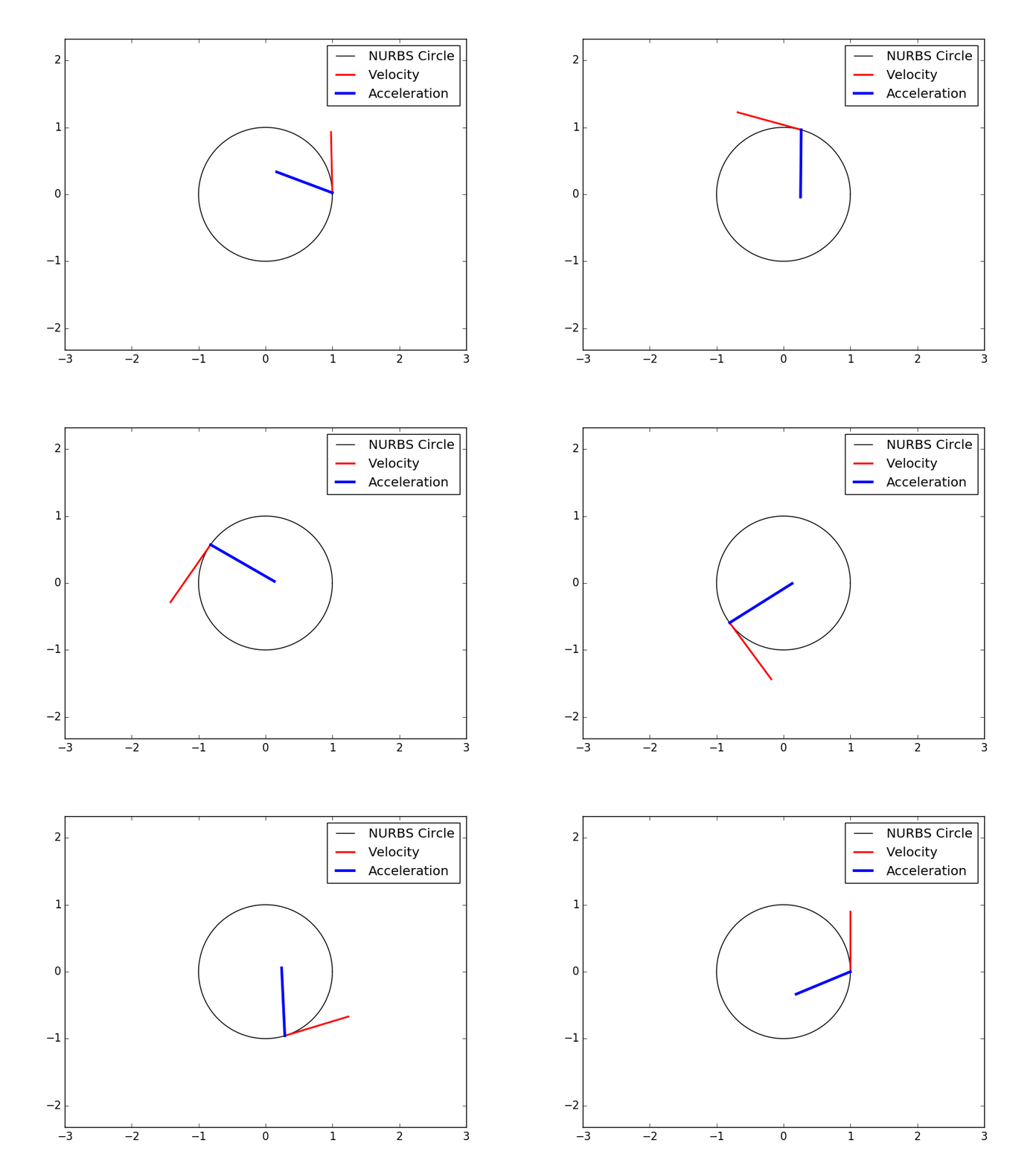
Derivatives of spline curves
  from splipy import *
  import numpy as np

  n = 250                                  # number of evaluation points
  c = curve_factory.circle()               # create the NURBS circle (r=1)
  t = np.linspace(c.start(0), c.end(0), n) # parametric evaluation points
  x = c(t)                                 # physical (x,y)-coordinates, size (n,2)
  v = c.derivative(t, 1)                   # velocity at all points
  a = c.derivative(t, 2)                   # acceleration at all points
Curve fitting
Lissajous curves are a family of parametric curves of the type
x = A sin(at+d)
y = B sin(bt)
More info: https://en.wikipedia.org/wiki/Lissajous_curve. Stripping the animation parts of the code, one can generate these curves in the following way
from splipy import *
import numpy as np
from fractions import gcd

def lissajous(a, b, d):
  # request a,b integers, so we have closed, periodic curves
  n = np.gcd(a,b)
  N = (a/n) * (b/n) # number of periods before looping

  # compute a set of interpolation points
  numb_pts = max(3*N, 100) # using 3N interpolation points is decent enough
  t = np.linspace(0,2*np.pi/n, numb_pts)
  x = np.array([np.sin(a*t + d), np.sin(b*t)])

# do a cubic curve interpolation with periodic boundary conditions
my_curve = curve_factory.cubic_curve(x.T, curve_factory.Boundary.PERIODIC)
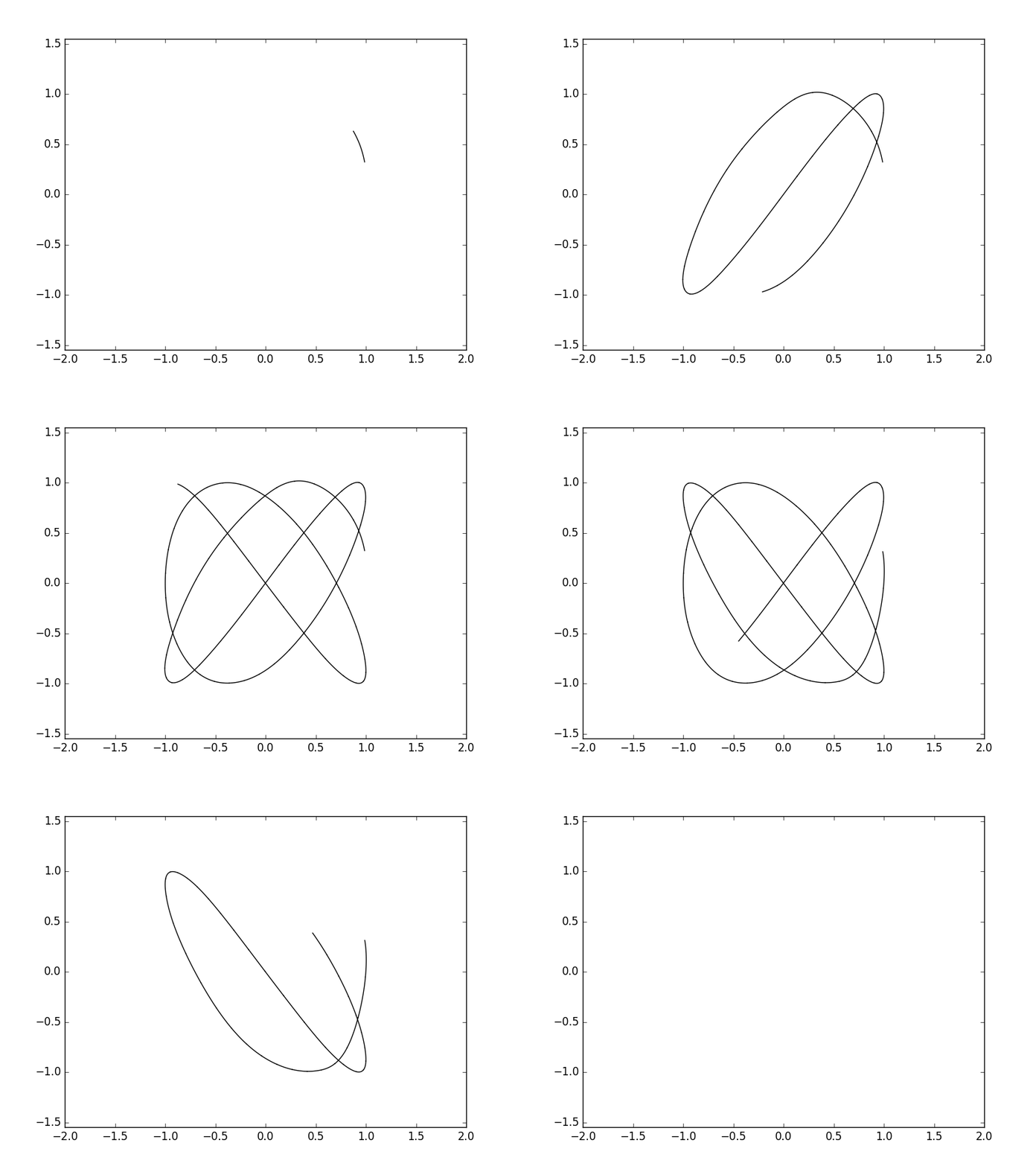
Animation of the lissajous curve with a=3, b=4 and d=pi/2
Surface Sweep
This produces the trefoil knot shown above
from splipy import *
from numpy import pi,cos,sin,transpose,array,sqrt

# define a parametric representation of the trefoil knot (to be sampled)
def trefoil(u):
  x = [41*cos(u) - 18*sin(  u) -  83*cos(2*u) - 83*sin(2*u) - 11*cos(3*u) + 27*sin(3*u),
       36*cos(u) + 27*sin(  u) - 113*cos(2*u) + 30*sin(2*u) + 11*cos(3*u) - 27*sin(3*u),
       45*sin(u) - 30*cos(2*u) + 113*sin(2*u) - 11*cos(3*u) + 27*sin(3*u)]
  return transpose(array(x))

knot_curve   = curve_factory.fit(trefoil, 0, 2*pi) # adaptive curve fit of trefoil knot
square_curve = 15 * curve_factory.n_gon(4)         # square cross-section
my_surface   = surface_factory.sweep(crv, square)  # sweep out the surface
Working with the controlpoints
>>> from splipy import *
>>> my_curve = curve_factory.circle(r=3)
>>> print(my_curve[0])
[3. 0. 1.]
>>> print(my_curve[1])
[2.12132034 2.12132034 0.70710678]
>>> for controlpoint in my_curve:
...     print(controlpoint)
[3. 0. 1.]
[2.12132034 2.12132034 0.70710678]
[0. 3. 1.]
[-2.12132034  2.12132034  0.70710678]
[-3.  0.  1.]
[-2.12132034 -2.12132034  0.70710678]
[ 0. -3.  1.]
[ 2.12132034 -2.12132034  0.70710678]
Creating STL files
STL files are used extensively for 3D representation and is one of the only supported formats for 3D printing.
from splipy.io import STL
from splipy import surface_factory

# create a NURBS torus
my_torus = surface_factory.torus(minor_r=1, major_r=4)

# STL files are tessellated linear triangles. View with i.e. meshlab
with STL('torus.stl') as my_file:
    my_file.write(my_torus, n=(50, 150)) # specify resolution of 50x150 evaluation pts
Torus tessellation as viewed in Meshlab

Citations
If you use Splipy in your work, please consider citing K. A. Johannessen and E. Fonn 2020 J. Phys.: Conf. Ser. 1669 012032.
2 maintainers


Release files for splipy 1.10.1
For a detailed explanation of source distributions (sdists) and built distributions (wheels), please see the package formats documentation.
Source distribution (sdist)
| File | Size | Uploaded | |
|---|---|---|---|
| splipy-1.10.1.tar.gz | 2.2 MB | Details |
Built distribution (wheel)
| File | Interpreter | ABI | Platform | Reset |
|---|---|---|---|---|
| splipy-1.10.1-py3-none-any.whl | Python 3 | none | any | Details |
Total release size: 2.3 MB
Release files / splipy-1.10.1.tar.gz
| Download URL | splipy-1.10.1.tar.gz |
|---|---|
| Size | 2.2 MB |
| Tags | Source |
|
SHA-256 checksum How to use checksums |
1fc4213142da1119d9f7b1bd69a10236ecfa3c236d9f1468635f532b35628095
|
|
BLAKE2b-256 checksum How to use checksums |
1cc737ed9cafdf502d6ed33ef7d9ed50f96606f6bf00a7f1b210bc3e60acfc20
|
| Upload date | |
|
Uploaded using Trusted Publishing? What is trusted publishing? |
No |
| Uploaded via |
twine/6.1.0 CPython/3.12.8
|
Release files / splipy-1.10.1-py3-none-any.whl
| Download URL | splipy-1.10.1-py3-none-any.whl |
|---|---|
| Size | 116.8 kB |
| Tags | Python 3 |
|
SHA-256 checksum How to use checksums |
f3ae7a1142e652a53bf845c98a059f26365312755d6d4431437ace1fdd42c620
|
|
BLAKE2b-256 checksum How to use checksums |
c11ba58637048ed59e79c6dc842a06593d92cca93a9be2fe236b5c18395d529e
|
| Upload date | |
|
Uploaded using Trusted Publishing? What is trusted publishing? |
No |
| Uploaded via |
twine/6.1.0 CPython/3.12.8
|














