Cielab color space

Project description
Cielab conversion tools
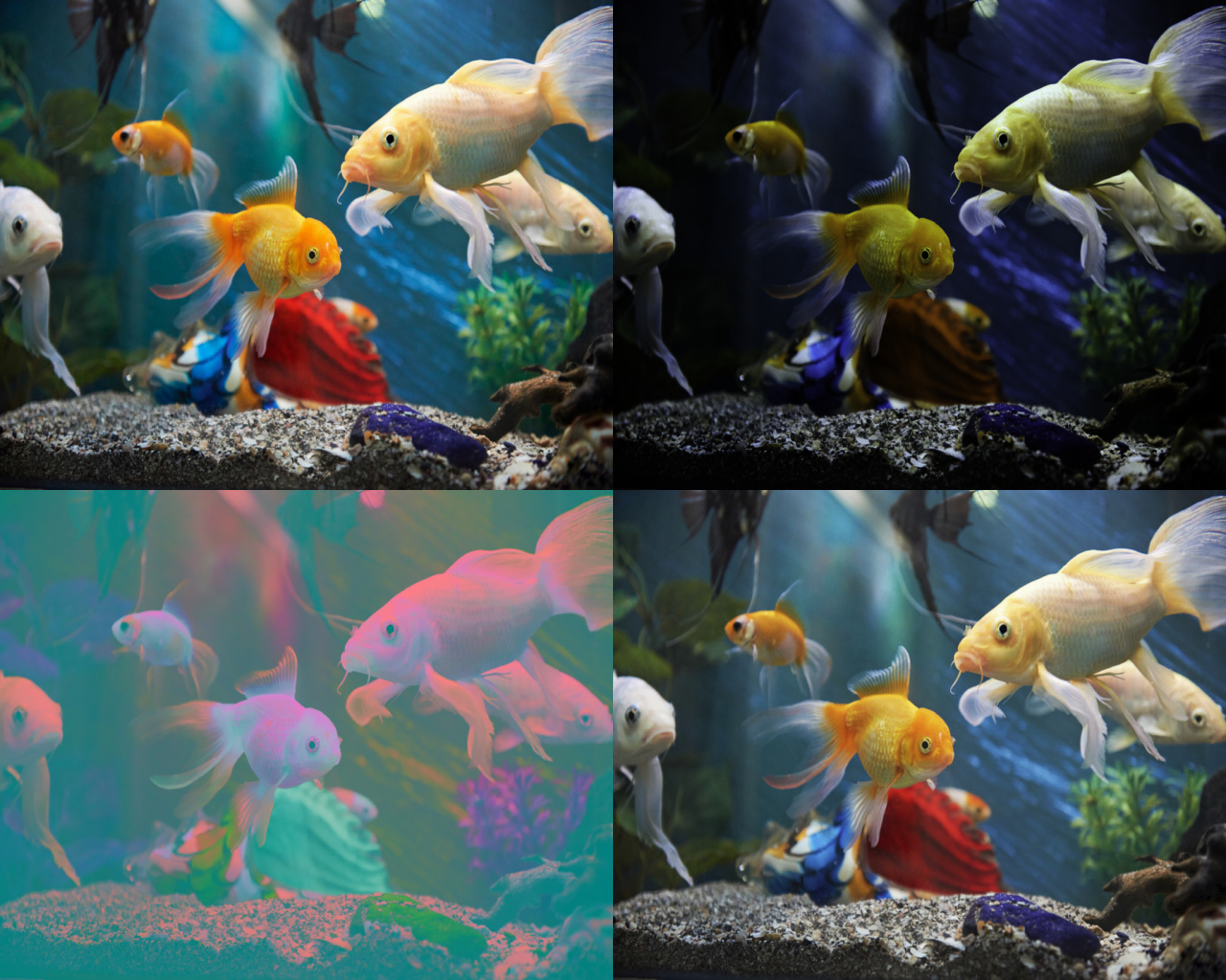
CIELAB is a free library coded with python and cython and offers fast conversion methods between various colour spaces such as sRGB, CIELAB, XYZ, ADOBE 98 and contains all the necessary methods to convert a color space domain from one to another and reciprocally.
This library is built with methods that can be call for a given pixel (RGB), LAB, XYZ tristimulus values, or used directly to an entire 3d arrays with similar color space.
Most of the image format such as PNG, JPEG, JPG, BMP etc will work with this library as long as you can provide a valid 3d array (refers to the methods arguments and documentations to pass a valid array shape and type). Check also the examples below that shows how to extract a 3d array from the most common known image processing library such as (OPENCV, PIL, scikit) or Pygame that provides very fast and efficient methods for image editing.
You can directly call Cielab conversion methods from your favourite Python editor
or choose to call the cythonized versions instead (only if you are familiar
with Cython). This will provide the best performances for your project(s).
Nevertheless, Cielab library offers both methods, Cython Cpdef hooks for
Python and cdef version for cython external library.
Most of the methods can be used with D50 and D65 illuminant used in the vast majority of industries and applications when using the Cielab pixel conversion methods.
Some useful color space definitions
What is Cielab (definition from Wikipedia)
The CIELAB color space, also referred to as Lab*, is a color space defined by the International Commission on Illumination (abbreviated CIE) in 1976. It expresses color as three values: L* for perceptual lightness and a* and b* for the four unique colors of human vision: red, green, blue and yellow.
The CIELAB space is three-dimensional and covers the entire gamut (range) of human color perception. It is based on the opponent color model of human vision, where red and green form an opponent pair and blue and yellow form an opponent pair. The lightness value, L*, also referred to as "Lstar", defines black at 0 and white at 100. The a* axis is relative to the green–red opponent colors, with negative values toward green and positive values toward red. The b* axis represents the blue–yellow opponents, with negative numbers toward blue and positive toward yellow.
The a* and b* axes are unbounded and depending on the reference white they can easily exceed ±150 to cover the human gamut. Nevertheless, software implementations often clamp these values for practical reasons. For instance, if integer math is being used it is common to clamp a* and b* in the range of −128 to 127.
CIELAB is calculated relative to a reference white, for which the CIE recommends the use of CIE Standard illuminant D65. D65 is used in the vast majority of industries and applications, with the notable exception being the printing industry which uses D50. The International Color Consortium largely supports the printing industry and uses D50 with either CIEXYZ or CIELAB in the Profile Connection Space, for v2 and v4 ICC profiles.
Meaning of X, Y and Z
The CIE 1931 RGB color space and CIE 1931 XYZ color space were created by the International Commission on Illumination (CIE) in 1931.They resulted from a series of experiments done in the late 1920s by William David Wright using ten observers and John Guild using seven observers. The experimental results were combined into the specification of the CIE RGB color space, from which the CIE XYZ color space was derived.
The CIE 1931 color spaces are still widely used, as is the 1976 CIELUV color space. Tristimulus values
The normalized spectral sensitivity of human cone cells of short-, middle- and long-wavelength types. The human eye with normal vision has three kinds of cone cells that sense light, having peaks of spectral sensitivity in short ("S", 420 nm – 440 nm), middle ("M", 530 nm – 540 nm), and long ("L", 560 nm – 580 nm) wavelengths. These cone cells underlie human color perception in conditions of medium and high brightness; in very dim light color vision diminishes, and the low-brightness, monochromatic "night vision" receptors, denominated "rod cells", become effective. Thus, three parameters corresponding to levels of stimulus of the three kinds of cone cells, in principle describe any human color sensation. Weighting a total light power spectrum by the individual spectral sensitivities of the three kinds of cone cells renders three effective values of stimulus; these three values compose a tristimulus specification of the objective color of the light spectrum. The three parameters, denoted "S", "M", and "L", are indicated using a 3-dimensional space denominated the "LMS color space", which is one of many color spaces devised to quantify human color vision.
A color space maps a range of physically produced colors from mixed light, pigments, etc. to an objective description of color sensations registered in the human eye, typically in terms of tristimulus values, but not usually in the LMS color space defined by the spectral sensitivities of the cone cells. The tristimulus values associated with a color space can be conceptualized as amounts of three primary colors in a tri-chromatic, additive color model. In some color spaces, including the LMS and XYZ spaces, the primary colors used are not real colors in the sense that they cannot be generated in any light spectrum.
The CIE XYZ color space encompasses all color sensations that are visible to a person with average eyesight. That is why CIE XYZ (Tristimulus values) is a device-invariant representation of color. It serves as a standard reference against which many other color spaces are defined. A set of color-matching functions, like the spectral sensitivity curves of the LMS color space, but not restricted to non-negative sensitivities, associates physically produced light spectra with specific tristimulus values.
Consider two light sources composed of different mixtures of various wavelengths. Such light sources may appear to be the same color; this effect is called "metamerism." Such light sources have the same apparent color to an observer when they produce the same tristimulus values, regardless of the spectral power distributions of the sources.
Most wavelengths stimulate two or all three kinds of cone cell because the spectral sensitivity curves of the three kinds overlap. Certain tristimulus values are thus physically impossible: e.g. LMS tristimulus values that are non-zero for the M component and zero for both the L and S components. Furthermore pure spectral colors would, in any normal trichromatic additive color space, e.g., the RGB color spaces, imply negative values for at least one of the three primaries because the chromaticity would be outside the color triangle defined by the primary colors. To avoid these negative RGB values, and to have one component that describes the perceived brightness, "imaginary" primary colors and corresponding color-matching functions were formulated. The CIE 1931 color space defines the resulting tristimulus values, in which they are denoted by "X", "Y", and "Z".In XYZ space, all combinations of non-negative coordinates are meaningful, but many, such as the primary locations [1, 0, 0], [0, 1, 0], and [0, 0, 1], correspond to imaginary colors outside the space of possible LMS coordinates; imaginary colors do not correspond to any spectral distribution of wavelengths and therefore have no physical reality.
Adobe RGB color space
The Adobe RGB (1998) color space or opRGB is a color space developed by Adobe Inc. in 1998. It was designed to encompass most of the colors achievable on CMYK color printers, but by using RGB primary colors on a device such as a computer display. The Adobe RGB (1998) color space encompasses roughly 30% of the visible colors specified by the CIELAB color space – improving upon the gamut of the sRGB color space, primarily in cyan-green hues. It was subsequently standardized by the IEC as IEC 61966-2-5:1999 with a name opRGB (optional RGB color space) and is used in HDMI.
SRGB
sRGB is a standard RGB (red, green, blue) color space that HP and Microsoft created cooperatively in 1996 to use on monitors, printers, and the World Wide Web. It was subsequently standardized by the International Electrotechnical Commission (IEC) as IEC 61966-2-1:1999. sRGB is the current defined standard colorspace for the web, and it is usually the assumed colorspace for images that are neither tagged for a colorspace nor have an embedded color profile.
sRGB essentially codifies the display specifications for the computer monitors in use at that time, which greatly aided its acceptance. sRGB uses the same color primaries and white point as ITU-R BT.709 standard for HDTV, a transfer function (or gamma) compatible with the era's CRT displays, and a viewing environment designed to match typical home and office viewing conditions.
Getting started:
Examples showing how to convert images
Pygame (convert RGB image to CIELAB)
WIDTH = 1280
HEIGHT = 1024
SCREEN = pygame.display.set_mode((WIDTH, HEIGHT))

# load an image
image = pygame.image.load("../Assets/background2.png")
rgb_array_ = pygame.surfarray.pixels3d(image)

# Transform an RGB array into CIELAB equivalent array using
# d65 illuminant
cielab_array = rgb_2_cielab(rgb_array_, illuminant ='d65', format_8b=False)
# Create a surface from the cielab array
image_cielab = pygame.surfarray.make_surface(cielab_array)
PIL (convert RGB image to CIELAB)
from PIL import Image
# load image
im = Image.open("../Assets/background2.png")
im_bytes = im.tobytes()

# create 3d array (682, 1024, 3) of type int8
rgb_array_ = numpy.frombuffer(im_bytes, dtype=numpy.uint8).reshape((682, 1024, 3))
# transpose width and height
rgb_array_ = rgb_array_.transpose(1, 0, 2).copy()
# Convert rgb array into cielab model
cielab_array = rgb_2_cielab(rgb_array_, illuminant ='d65', format_8b=False)

cielab_array = cielab_array.transpose(1, 0, 2)
numpy.ndarray.flatten(cielab_array)

image_str = (cielab_array.astype(numpy.uint8)).tobytes()
image = Image.frombytes('RGB', (1024, 682), image_str)
image.show()
PIL (convert RGB image to ADOBE 98)
from PIL import Image
# load image
im = Image.open("../Assets/background2.png")
im_bytes = im.tobytes()

# create 3d array (682, 1024, 3) of type int8
rgb_array_ = numpy.frombuffer(im_bytes, dtype=numpy.uint8).reshape((682, 1024, 3))
# transpose width and height
rgb_array_ = rgb_array_.transpose(1, 0, 2).copy()
# Convert rgb array into adobe98 array using d65 illuminant
adobe_array = rgb2adobe(rgb_array_, ref ='d65')

adobe_array = adobe_array.transpose(1, 0, 2)
numpy.ndarray.flatten(adobe_array)

image_str = (adobe_array.astype(numpy.uint8)).tobytes()
image = Image.frombytes('RGB', (1024, 682), image_str)
image.show()
OpenCv (convert RGB image to CIELAB)
import cv2
img = cv2.imread("../Assets/background2.png")
cielab_array = rgb_2_cielab(img, illuminant ='d65', format_8b=False)
cielab_array = cv2.cvtColor(cielab_array, cv2.COLOR_BGR2RGB)
cv2.imshow('image', cielab_array.astype(numpy.uint8))
cv2.waitKey(0)
cv2.destroyAllWindows()
scikit-image (convert RGB image to CIELAB)
import skimage as ski
import os
import matplotlib
from matplotlib import pyplot as plt
matplotlib.use('TkAgg')
filename = os.path.join(ski.data_dir, '../Assets/background2.png')
rgb_array = ski.io.imread(filename)
rgb_array = rgb_array.transpose(1, 0, 2)
cielab_array = rgb_2_cielab(rgb_array, illuminant ='d50', format_8b=False)
image = cielab_array.transpose(1, 0, 2).astype(numpy.uint8)
plt.imshow(image)
plt.show()
Example showing how to convert color information
# Color definition
# RGB 255.0 0 0 (RED)
# XYZ 41.246 | 21.267 | 1.933
# Adobe 218.946 0 0.048
x, y, z = 41.246, 21.267, 1.933

# XYZ to ADOBE 98
r, g, b = xyz_adobe98(x, y, z, ref='D65').values()
# RGB to XYZ
x, y, z = rgb_to_xyz(255.0, 0, 0).values()  # default d65
# XYZ to CIELAB
D65 = numpy.array([0.9504, 1.0000, 1.0888], dtype=float32)
l, a, b = xyz_to_cielab(
   41.24563980102539,
   21.267290115356445,
   1.9333901405334473, model=D65).values()
Array mean and standard deviation
import skimage as ski
import os
import matplotlib
from matplotlib import pyplot as plt
matplotlib.use('TkAgg')
filename = os.path.join(ski.data_dir, '../Assets/background2.png')
rgb_array = ski.io.imread(filename)
# Get RGB mean and standard deviation for each channels
red_mean, red_dev, \
green_mean, green_dev,\
blue_mean, blue_dev = array3d_stats(rgb_array).values()
PIXEL TRANSFORMATION
Convert XYZ tristimulus to ADOBE98 and back (D65 or D50 illuminant)
xyz_adobe98(x, y, z, ref='D65')

adobe98_xyz(r, g, b, ref='D65')
Convert RGB to XYZ tristimulus and back (D65 or D50 illuminant)
rgb_to_xyz(r, g, b, ref='D65')

xyz_to_rgb( x, y, z, ref='D65')
Convert XYZ to CIELAB and back; models ('a', 'c', 'e', 'd50', 'd55', 'd65', 'icc')
xyz_to_cielab(x, y, z, model=model_d65, format_8b = False)

cielab_to_xyz(l , a, b, model=model_d65, format_8b = False)
Convert RGB to CIELAB and back; models ('a', 'c', 'e', 'd50', 'd55', 'd65', 'icc')
rgb_to_cielab(r, g, b, model=model_d65, format_8b = False)

cielab_to_rgb(l, a, b, model=model_d65, format_8b = False)
ARRAY TRANSFORMATION
Convert ARRAY RGB to ARRAY CIELAB; models ('a', 'c', 'e', 'd50', 'd55', 'd65', 'icc')
rgb_2_cielab(rgb_array_, illuminant_ ='d65', format_8b=False)

cielab_2_rgb(lab_array_, illuminant_ ='d65', format_8b=False)
White balance ; models ('a', 'c', 'e', 'd50', 'd55', 'd65', 'icc')
WhiteBalance(rgb_array_, c1=1.0, illuminant_='D65', format_8b = False)

WhiteBalanceInplace(rgb_array_,  c1=1.0, illuminant_='D65', format_8b = False)
ADOBE98 ARRAY to RGB ARRAY and back ; models ('d50', 'd65')
adobe2rgb(adobe98_array_, ref='D65')

rgb2adobe(rgb_array_, ref='D65')

rgb2adobe_inplace(rgb_array_, ref='D65')

adobe2rgb_inplace(adobe98_array_, ref='D65')
RGB array to XYZ array ; models ('d50', 'd65')
rgb2xyz(rgb_array_, ref='D65')
In python Idle
from Cielab import *
Installation from pip
Check the link for newest version https://pypi.org/project/Cielab/
From the command line
C:\>pip install Cielab
Credit
Yoann Berenguer
Dependencies :
numpy >= 1.19.5
pygame ==2.5.2
cython =>3.0.2
setuptools~=54.1.1
License :
GNU GENERAL PUBLIC LICENSE Version 3
Copyright (c) 2019 Yoann Berenguer
Copyright (C) 2007 Free Software Foundation, Inc. https://fsf.org/ Everyone is permitted to copy and distribute verbatim copies of this license document, but changing it is not allowed.
Testing:
>>> import Cielab
>>> from Cielab.tests.test_cielab import run_testsuite
>>> run_testsuite()
Performances:
From the command line
C:\>cd tests
C:\>python profiler.py
Release history Release notifications | RSS feed

Download files
Download the file for your platform. If you're not sure which to choose, learn more about installing packages.
Source Distribution
Built Distributions
Filter files by name, interpreter, ABI, and platform.
If you're not sure about the file name format, learn more about wheel file names.
Copy a direct link to the current filters
File details
Details for the file Cielab-1.0.0.tar.gz.
File metadata
- Download URL: Cielab-1.0.0.tar.gz
- Upload date:
- Size: 6.0 MB
- Tags: Source
- Uploaded using Trusted Publishing? No
- Uploaded via: twine/5.0.0 CPython/3.12.2
File hashes
| Algorithm | Hash digest | |
|---|---|---|
| SHA256 |
35399415267a3ddb836ef83b50da9150e24893ca1b8419cb94ca75a0cf063c1e
|
|
| MD5 |
9f834573d29c111e3439b08da88169a8
|
|
| BLAKE2b-256 |
97e787fa0ddba0ed237a6bd8292923b77771ac671c429ee71c004ddaad73d828
|
File details
Details for the file Cielab-1.0.0-cp312-cp312-win_amd64.whl.
File metadata
- Download URL: Cielab-1.0.0-cp312-cp312-win_amd64.whl
- Upload date:
- Size: 11.9 MB
- Tags: CPython 3.12, Windows x86-64
- Uploaded using Trusted Publishing? No
- Uploaded via: twine/5.0.0 CPython/3.12.2
File hashes
| Algorithm | Hash digest | |
|---|---|---|
| SHA256 |
e39b2f99fc5eaf2531b98ca1cd8a925c5f1f1b01a10ade71b9724a110b658aec
|
|
| MD5 |
9284e5130cb87340ad0e4e360edc6939
|
|
| BLAKE2b-256 |
6bbcd909e59b22dba5dc96a3ddf0a2afe541e178d00bf18340e3b3e2a8fef893
|
File details
Details for the file Cielab-1.0.0-cp312-cp312-win32.whl.
File metadata
- Download URL: Cielab-1.0.0-cp312-cp312-win32.whl
- Upload date:
- Size: 11.9 MB
- Tags: CPython 3.12, Windows x86
- Uploaded using Trusted Publishing? No
- Uploaded via: twine/5.0.0 CPython/3.12.2
File hashes
| Algorithm | Hash digest | |
|---|---|---|
| SHA256 |
ad9d13922e4dc7bcc7f15c91aea76258379cb3fa3a64c5b18ff04538c2f0b76f
|
|
| MD5 |
c85d8bccde1f1de6706257bae6353d51
|
|
| BLAKE2b-256 |
946dfa7d4bc8c5c57cfac86c9440a27217095b591d4c199d1ed16e2841c534ea
|
File details
Details for the file Cielab-1.0.0-cp311-cp311-win_amd64.whl.
File metadata
- Download URL: Cielab-1.0.0-cp311-cp311-win_amd64.whl
- Upload date:
- Size: 11.9 MB
- Tags: CPython 3.11, Windows x86-64
- Uploaded using Trusted Publishing? No
- Uploaded via: twine/5.0.0 CPython/3.12.2
File hashes
| Algorithm | Hash digest | |
|---|---|---|
| SHA256 |
4de8935eaf721c7620189f815c1a9bfded4ff3358f0d65806f4e7882b8439d68
|
|
| MD5 |
44a10b1f7633244ac5241a277f969da8
|
|
| BLAKE2b-256 |
01af116d622ce4e2e16b2b5ea89bb453a8487666d85fb6219fd918be908a19a4
|
File details
Details for the file Cielab-1.0.0-cp311-cp311-win32.whl.
File metadata
- Download URL: Cielab-1.0.0-cp311-cp311-win32.whl
- Upload date:
- Size: 11.9 MB
- Tags: CPython 3.11, Windows x86
- Uploaded using Trusted Publishing? No
- Uploaded via: twine/5.0.0 CPython/3.12.2
File hashes
| Algorithm | Hash digest | |
|---|---|---|
| SHA256 |
52d813b147b985b0fa558a8f92389a393078ee3540a3c849b057cc2b7e4ae3c9
|
|
| MD5 |
3112077e18c4cb6680633f84265fe09e
|
|
| BLAKE2b-256 |
9f6a57d8b72a3e6684a2aa75a6acdb1dc20aac296e0d683ff21867901a11cf63
|
File details
Details for the file Cielab-1.0.0-cp311-cp311-manylinux_2_24_x86_64.whl.
File metadata
- Download URL: Cielab-1.0.0-cp311-cp311-manylinux_2_24_x86_64.whl
- Upload date:
- Size: 12.4 MB
- Tags: CPython 3.11, manylinux: glibc 2.24+ x86-64
- Uploaded using Trusted Publishing? No
- Uploaded via: twine/5.0.0 CPython/3.12.2
File hashes
| Algorithm | Hash digest | |
|---|---|---|
| SHA256 |
7ae8770a1f88e316633fdc10e82bc60d9989668855e47dd62b8c008499958b99
|
|
| MD5 |
336a4aea4fb9a777c854adac527e3697
|
|
| BLAKE2b-256 |
e001ce5295a1e345043c4d7bd1d42d413e959eb7d931cf4d61ddd48d9ef99e87
|
File details
Details for the file Cielab-1.0.0-cp311-cp311-manylinux_2_24_i686.whl.
File metadata
- Download URL: Cielab-1.0.0-cp311-cp311-manylinux_2_24_i686.whl
- Upload date:
- Size: 12.3 MB
- Tags: CPython 3.11, manylinux: glibc 2.24+ i686
- Uploaded using Trusted Publishing? No
- Uploaded via: twine/5.0.0 CPython/3.12.2
File hashes
| Algorithm | Hash digest | |
|---|---|---|
| SHA256 |
895bf6e998dc6ee8a4a2c1474f1c0bc1c04b6da38543b84c4e22882a08b14d7b
|
|
| MD5 |
165ec0be8071cc45f535e4eea7cd9982
|
|
| BLAKE2b-256 |
a88b15945a535397d9b3371685d29684bfc547dbd1eca13928a40187872d4347
|
File details
Details for the file Cielab-1.0.0-cp310-cp310-win_amd64.whl.
File metadata
- Download URL: Cielab-1.0.0-cp310-cp310-win_amd64.whl
- Upload date:
- Size: 11.9 MB
- Tags: CPython 3.10, Windows x86-64
- Uploaded using Trusted Publishing? No
- Uploaded via: twine/5.0.0 CPython/3.12.2
File hashes
| Algorithm | Hash digest | |
|---|---|---|
| SHA256 |
9b24933373f66f62d12fb36da4ab8b05d40e772526808f2a91233139d7e78e56
|
|
| MD5 |
bf15737cef0156377d52be7de63d2ce2
|
|
| BLAKE2b-256 |
3feb2bcd1d3921e4c659ca028a1d99b55b12a2c9e67b30471adf861531117baf
|
File details
Details for the file Cielab-1.0.0-cp310-cp310-win32.whl.
File metadata
- Download URL: Cielab-1.0.0-cp310-cp310-win32.whl
- Upload date:
- Size: 11.9 MB
- Tags: CPython 3.10, Windows x86
- Uploaded using Trusted Publishing? No
- Uploaded via: twine/5.0.0 CPython/3.12.2
File hashes
| Algorithm | Hash digest | |
|---|---|---|
| SHA256 |
c598f035df736ad545b834d184fe302c635c0353d94aea12ac46600e4432f164
|
|
| MD5 |
4767c58b88ead9bfe5cdeba77a7fd151
|
|
| BLAKE2b-256 |
0ece01295e8132ae10104c7d5376aeea97b0ea161c1a58518b3f0d1ec6acca9f
|
File details
Details for the file Cielab-1.0.0-cp310-cp310-manylinux_2_24_x86_64.whl.
File metadata
- Download URL: Cielab-1.0.0-cp310-cp310-manylinux_2_24_x86_64.whl
- Upload date:
- Size: 12.3 MB
- Tags: CPython 3.10, manylinux: glibc 2.24+ x86-64
- Uploaded using Trusted Publishing? No
- Uploaded via: twine/5.0.0 CPython/3.12.2
File hashes
| Algorithm | Hash digest | |
|---|---|---|
| SHA256 |
df49ee772d58fead43e0af04ee2488f6573b7725d596bbbd6dacf4617a4e2d39
|
|
| MD5 |
774ffa6a018978fde2704b5a2e7aff84
|
|
| BLAKE2b-256 |
1f1a55c061cff860c5a85c8397fa2303a69eacd5f0c7495ee7a6e32de073128b
|
File details
Details for the file Cielab-1.0.0-cp310-cp310-manylinux_2_24_i686.whl.
File metadata
- Download URL: Cielab-1.0.0-cp310-cp310-manylinux_2_24_i686.whl
- Upload date:
- Size: 12.3 MB
- Tags: CPython 3.10, manylinux: glibc 2.24+ i686
- Uploaded using Trusted Publishing? No
- Uploaded via: twine/5.0.0 CPython/3.12.2
File hashes
| Algorithm | Hash digest | |
|---|---|---|
| SHA256 |
677bca1a46dbe1b0ca441bb265758deb4c182aeef6660248036de8db049a3133
|
|
| MD5 |
f05c2526a6a95e0c28d360feff538b0f
|
|
| BLAKE2b-256 |
0da439131133e7069560d115a00276cac9560752799ad0a32b0040aa28ed98cb
|
File details
Details for the file Cielab-1.0.0-cp39-cp39-win_amd64.whl.
File metadata
- Download URL: Cielab-1.0.0-cp39-cp39-win_amd64.whl
- Upload date:
- Size: 11.9 MB
- Tags: CPython 3.9, Windows x86-64
- Uploaded using Trusted Publishing? No
- Uploaded via: twine/5.0.0 CPython/3.12.2
File hashes
| Algorithm | Hash digest | |
|---|---|---|
| SHA256 |
a09c51fb8f1dcfe5815f9f1f1a038f4772821af80dd3c4df95623a0fccef7025
|
|
| MD5 |
5a42761c7a16001c3c10eca1aa361b43
|
|
| BLAKE2b-256 |
58387e62f0f96aca7e0f207039e59892d8076ddb1c074f21613ee99cd747ad90
|
File details
Details for the file Cielab-1.0.0-cp39-cp39-win32.whl.
File metadata
- Download URL: Cielab-1.0.0-cp39-cp39-win32.whl
- Upload date:
- Size: 11.9 MB
- Tags: CPython 3.9, Windows x86
- Uploaded using Trusted Publishing? No
- Uploaded via: twine/5.0.0 CPython/3.12.2
File hashes
| Algorithm | Hash digest | |
|---|---|---|
| SHA256 |
b5af0efcd3e3cfbf1668dbf30f3a7c50e27bd07b93efc9f0947846590b033d21
|
|
| MD5 |
651311538017805b7df3a65ce1ca68eb
|
|
| BLAKE2b-256 |
c6cca88e979618f0c9c524bc2706228067c150d95d209e3d0eb8237ae5f02a8a
|
File details
Details for the file Cielab-1.0.0-cp39-cp39-manylinux_2_24_x86_64.whl.
File metadata
- Download URL: Cielab-1.0.0-cp39-cp39-manylinux_2_24_x86_64.whl
- Upload date:
- Size: 12.3 MB
- Tags: CPython 3.9, manylinux: glibc 2.24+ x86-64
- Uploaded using Trusted Publishing? No
- Uploaded via: twine/5.0.0 CPython/3.12.2
File hashes
| Algorithm | Hash digest | |
|---|---|---|
| SHA256 |
28306166c85cde925fb3f7445832ea89cbec55861a4afb702c2cc321408270a9
|
|
| MD5 |
60dc3f311f6893ad8b3da6e59fdd1eea
|
|
| BLAKE2b-256 |
3628f5ae4057523d67c8a5843c6cd782b4f29e7af9bd415e2c184497379a8007
|
File details
Details for the file Cielab-1.0.0-cp39-cp39-manylinux_2_24_i686.whl.
File metadata
- Download URL: Cielab-1.0.0-cp39-cp39-manylinux_2_24_i686.whl
- Upload date:
- Size: 12.3 MB
- Tags: CPython 3.9, manylinux: glibc 2.24+ i686
- Uploaded using Trusted Publishing? No
- Uploaded via: twine/5.0.0 CPython/3.12.2
File hashes
| Algorithm | Hash digest | |
|---|---|---|
| SHA256 |
76b1e273eebab9ae6dbc2d8fc7ebcf158638cfbc0f720727760c53eeed26d704
|
|
| MD5 |
056a23c64598d9de2ce037829da3d2b6
|
|
| BLAKE2b-256 |
07d32796a46d8421954f6d192c565c414e8cb620fa5f7cf77ac65dc7bf7326e2
|
File details
Details for the file Cielab-1.0.0-cp38-cp38-win_amd64.whl.
File metadata
- Download URL: Cielab-1.0.0-cp38-cp38-win_amd64.whl
- Upload date:
- Size: 11.9 MB
- Tags: CPython 3.8, Windows x86-64
- Uploaded using Trusted Publishing? No
- Uploaded via: twine/5.0.0 CPython/3.12.2
File hashes
| Algorithm | Hash digest | |
|---|---|---|
| SHA256 |
a3d994327f6f06fca5992b0acf961bf0f4c4b8c98291a88037d7e34839621d0b
|
|
| MD5 |
d94e4da542470a2a4a89da9dd838e15e
|
|
| BLAKE2b-256 |
9456915ce5dda35f77eea6dea1ffd6e4c3a749551d522bad21b8ed6c5634931f
|
File details
Details for the file Cielab-1.0.0-cp38-cp38-win32.whl.
File metadata
- Download URL: Cielab-1.0.0-cp38-cp38-win32.whl
- Upload date:
- Size: 11.9 MB
- Tags: CPython 3.8, Windows x86
- Uploaded using Trusted Publishing? No
- Uploaded via: twine/5.0.0 CPython/3.12.2
File hashes
| Algorithm | Hash digest | |
|---|---|---|
| SHA256 |
230c698505eef1bb8b49a690e42af5eacde068fba1bbd30f016ba8f75876800e
|
|
| MD5 |
1e18e4fdc88e4e2615cc8e107d43f1f8
|
|
| BLAKE2b-256 |
b74c674fc3985822fb059fec019b514f99da71af1b92fffd8fa7482d2e9cfbf5
|
File details
Details for the file Cielab-1.0.0-cp38-cp38-manylinux_2_24_x86_64.whl.
File metadata
- Download URL: Cielab-1.0.0-cp38-cp38-manylinux_2_24_x86_64.whl
- Upload date:
- Size: 12.4 MB
- Tags: CPython 3.8, manylinux: glibc 2.24+ x86-64
- Uploaded using Trusted Publishing? No
- Uploaded via: twine/5.0.0 CPython/3.12.2
File hashes
| Algorithm | Hash digest | |
|---|---|---|
| SHA256 |
07959d59abf4c2dc02ce66609a664948b9fbf1e2f1882a9ac724e9d08ba63397
|
|
| MD5 |
fb688db7b0c409c062aaf1bb9d77a410
|
|
| BLAKE2b-256 |
9c023cfed06b8fde2cdbea8cfe243c3c6dd1ddd02e080be0114775e7e05566e1
|
File details
Details for the file Cielab-1.0.0-cp38-cp38-manylinux_2_24_i686.whl.
File metadata
- Download URL: Cielab-1.0.0-cp38-cp38-manylinux_2_24_i686.whl
- Upload date:
- Size: 12.3 MB
- Tags: CPython 3.8, manylinux: glibc 2.24+ i686
- Uploaded using Trusted Publishing? No
- Uploaded via: twine/5.0.0 CPython/3.12.2
File hashes
| Algorithm | Hash digest | |
|---|---|---|
| SHA256 |
2e9375db8b9f4f449a419c373e79b80fca8d8ea3db3682cbfb9bdf143cf16781
|
|
| MD5 |
8677f41a000950f65b6375f0842b884b
|
|
| BLAKE2b-256 |
4d0646989d7f97f82c167d26f6f162d9cc5f0716f70c078dce0d1c23b9cdef05
|
File details
Details for the file Cielab-1.0.0-cp37-cp37m-win_amd64.whl.
File metadata
- Download URL: Cielab-1.0.0-cp37-cp37m-win_amd64.whl
- Upload date:
- Size: 11.9 MB
- Tags: CPython 3.7m, Windows x86-64
- Uploaded using Trusted Publishing? No
- Uploaded via: twine/5.0.0 CPython/3.12.2
File hashes
| Algorithm | Hash digest | |
|---|---|---|
| SHA256 |
ee64dd43a0829ac75bead0656a0bbc88f02fa922f9a31024467aced9a92c9b9e
|
|
| MD5 |
c26ea8bda224e2238a74484981a482d0
|
|
| BLAKE2b-256 |
140772f00a6672d2c115641a8090b4abacf0b697e976b49f99d14f8eeb90e161
|
File details
Details for the file Cielab-1.0.0-cp37-cp37m-win32.whl.
File metadata
- Download URL: Cielab-1.0.0-cp37-cp37m-win32.whl
- Upload date:
- Size: 11.9 MB
- Tags: CPython 3.7m, Windows x86
- Uploaded using Trusted Publishing? No
- Uploaded via: twine/5.0.0 CPython/3.12.2
File hashes
| Algorithm | Hash digest | |
|---|---|---|
| SHA256 |
144a8a86ca33fca2c9326088b8d556bd6a351ad4bfacc439dd55df1c5a52e056
|
|
| MD5 |
c9c7f8f7ece4b18ecda075c01bdb3f45
|
|
| BLAKE2b-256 |
36739fe7f88aa9da6d944d84ca5208615db492aea1a0143e1904f75b92214f48
|
File details
Details for the file Cielab-1.0.0-cp37-cp37m-manylinux_2_24_x86_64.whl.
File metadata
- Download URL: Cielab-1.0.0-cp37-cp37m-manylinux_2_24_x86_64.whl
- Upload date:
- Size: 12.3 MB
- Tags: CPython 3.7m, manylinux: glibc 2.24+ x86-64
- Uploaded using Trusted Publishing? No
- Uploaded via: twine/5.0.0 CPython/3.12.2
File hashes
| Algorithm | Hash digest | |
|---|---|---|
| SHA256 |
d2f10920537f4ef7cf7ea9614f0d8dcd95167b3e8ad21fad91a95528ea145015
|
|
| MD5 |
f90b119f32ad7aa005f6255282730d90
|
|
| BLAKE2b-256 |
775ad73a7be7402a4d8794ea17281968241d1a004c59081a0d4687f32fa91df2
|
File details
Details for the file Cielab-1.0.0-cp37-cp37m-manylinux_2_24_i686.whl.
File metadata
- Download URL: Cielab-1.0.0-cp37-cp37m-manylinux_2_24_i686.whl
- Upload date:
- Size: 12.3 MB
- Tags: CPython 3.7m, manylinux: glibc 2.24+ i686
- Uploaded using Trusted Publishing? No
- Uploaded via: twine/5.0.0 CPython/3.12.2
File hashes
| Algorithm | Hash digest | |
|---|---|---|
| SHA256 |
5a823da821736bf8e40a22a086e1048ef8dd89e1d5ea7f377c4686b0554b4fde
|
|
| MD5 |
e6c375adee578700d90d2169ab8a6b59
|
|
| BLAKE2b-256 |
068a4aad558f06ac95d0e6b604ee99ee822c611ef3aee5b591f316450c2c02c5
|
File details
Details for the file Cielab-1.0.0-cp36-cp36m-win_amd64.whl.
File metadata
- Download URL: Cielab-1.0.0-cp36-cp36m-win_amd64.whl
- Upload date:
- Size: 11.9 MB
- Tags: CPython 3.6m, Windows x86-64
- Uploaded using Trusted Publishing? No
- Uploaded via: twine/5.0.0 CPython/3.12.2
File hashes
| Algorithm | Hash digest | |
|---|---|---|
| SHA256 |
41b58924b7605ff8e0d2d66c4ae552e8acc8cd9a23c28971403f454f3cc1404c
|
|
| MD5 |
86a76762b352be1ca23dc047b4e59d02
|
|
| BLAKE2b-256 |
48f1297e8d4a55a0d35b18af3f0d3907eac720f751a6894309cc22b221e60f69
|
File details
Details for the file Cielab-1.0.0-cp36-cp36m-win32.whl.
File metadata
- Download URL: Cielab-1.0.0-cp36-cp36m-win32.whl
- Upload date:
- Size: 11.9 MB
- Tags: CPython 3.6m, Windows x86
- Uploaded using Trusted Publishing? No
- Uploaded via: twine/5.0.0 CPython/3.12.2
File hashes
| Algorithm | Hash digest | |
|---|---|---|
| SHA256 |
5d21923ed9d1c8fa3f6a4f46ad7613c9311951eba0df738adb5bc4202770533d
|
|
| MD5 |
07fed13bd162a77c3fdc903b14f80280
|
|
| BLAKE2b-256 |
63eb92bc5fabe07190e119efd7da9dfc3e9ea4ce18bf6078f95acedc6478fc3d
|
File details
Details for the file Cielab-1.0.0-cp36-cp36m-manylinux_2_24_x86_64.whl.
File metadata
- Download URL: Cielab-1.0.0-cp36-cp36m-manylinux_2_24_x86_64.whl
- Upload date:
- Size: 12.3 MB
- Tags: CPython 3.6m, manylinux: glibc 2.24+ x86-64
- Uploaded using Trusted Publishing? No
- Uploaded via: twine/5.0.0 CPython/3.12.2
File hashes
| Algorithm | Hash digest | |
|---|---|---|
| SHA256 |
ed46d3b05ec6883b9150aeabb4cb49cfaa19fa5ee01aaaa6430f4ccb5c26e05e
|
|
| MD5 |
19c8df14a068b17ad6d63a46005575e2
|
|
| BLAKE2b-256 |
19a64cbf8aa7b7993060d3d60c804dc2f8bc5f8d11bd2613c3db7475229db41d
|
File details
Details for the file Cielab-1.0.0-cp36-cp36m-manylinux_2_24_i686.whl.
File metadata
- Download URL: Cielab-1.0.0-cp36-cp36m-manylinux_2_24_i686.whl
- Upload date:
- Size: 12.3 MB
- Tags: CPython 3.6m, manylinux: glibc 2.24+ i686
- Uploaded using Trusted Publishing? No
- Uploaded via: twine/5.0.0 CPython/3.12.2
File hashes
| Algorithm | Hash digest | |
|---|---|---|
| SHA256 |
5e4121b678dc822b476b542df7ddf7b9a17f6bb8f966345675fc9de3cd35f2e2
|
|
| MD5 |
05017bc26af8310aec6aec428da19358
|
|
| BLAKE2b-256 |
c47545e6b73eb729165f54d8d0e49e40be8533a2bc1286c28317ac1736750b06
|


