An easy implementation of genetic-algorithm (GA) to solve continuous and combinatorial optimization problems with real, integer, and mixed variables in Python

Project description
geneticalgorithm
geneticalgorithm is a Python library distributed on Pypi for implementing standard and elitist genetic-algorithm (GA). This package solves continuous, combinatorial and mixed optimization problems with continuous, discrete, and mixed variables. It provides an easy implementation of genetic-algorithm (GA) in Python.
Installation
Use the package manager pip to install geneticalgorithm in Python.
pip install geneticalgorithm
version 1.0.2 updates
@param convergence_curve <True/False> - Plot the convergence curve or not. Default is True. @param progress_bar <True/False> - Show progress bar or not. Default is True.
A simple example
Assume we want to find a set of X=(x1,x2,x3) that minimizes function f(X)=x1+x2+x3 where X can be any real number in [0,10].
This is a trivial problem and we already know that the answer is X=(0,0,0) where f(X)=0.
We just use this simple example to see how to implement geneticalgorithm:
First we import geneticalgorithm and numpy. Next, we define function f which we want to minimize and the boundaries of the decision variables; Then simply geneticalgorithm is called to solve the defined optimization problem as follows:
import numpy as np
from geneticalgorithm import geneticalgorithm as ga

def f(X):
    return np.sum(X)


varbound=np.array([[0,10]]*3)

model=ga(function=f,dimension=3,variable_type='real',variable_boundaries=varbound)

model.run()
Notice that we define the function f so that its output is the objective function we want to minimize where the input is the set of X (decision variables). The boundaries for variables must be defined as a numpy array and for each variable we need a separate boundary. Here I have three variables and all of them have the same boundaries (For the case the boundaries are different see the example with mixed variables).
geneticalgorithm has some arguments:
Obviously the first argument is the function f we already defined (for more details about the argument and output see Function).
Our problem has three variables so we set dimension equal three.
Variables are real (continuous) so we use string 'real' to notify the type of
variables (geneticalgorithm accepts other types including Boolean, Integers and
Mixed; see other examples).
Finally, we input varbound which includes the boundaries of the variables.
Note that the length of variable_boundaries must be equal to dimension.
If you run the code, you should see a progress bar that shows the progress of the genetic algorithm (GA) and then the solution, objective function value and the convergence curve as follows:

Also we can access to the best answer of the defined optimization problem found by geneticalgorithm as a dictionary and a report of the progress of the genetic algorithm. To do so we complete the code as follows:
convergence=model.report
solution=model.ouput_dict
output_dict is a dictionary including the best set of variables found and the value of the given function associated to it ({'variable': , 'function': }). report is a list including the convergence of the algorithm over iterations
The simple example with integer variables
Considering the problem given in the simple example above. Now assume all variables are integers. So x1, x2, x3 can be any integers in [0,10]. In this case the code is as the following:
import numpy as np
from geneticalgorithm import geneticalgorithm as ga

def f(X):
    return np.sum(X)


varbound=np.array([[0,10]]*3)

model=ga(function=f,dimension=3,variable_type='int',variable_boundaries=varbound)

model.run()
So, as it is seen the only difference is that for variable_type we use string 'int'.
The simple example with Boolean variables
Considering the problem given in the simple example above. Now assume all variables are Boolean instead of real or integer. So X can be either zero or one. Also instead of three let's have 30 variables. In this case the code is as the following:
import numpy as np
from geneticalgorithm import geneticalgorithm as ga

def f(X):
    return np.sum(X)


model=ga(function=f,dimension=30,variable_type='bool')

model.run()
Note for variable_type we use string 'bool' when all variables are Boolean.
Note that when variable_type equal 'bool' there is no need for variable_boundaries to be defined.
The simple example with mixed variables
Considering the problem given in the the simple example above where we want to minimize f(X)=x1+x2+x3. Now assume x1 is a real (continuous) variable in [0.5,1.5], x2 is an integer variable in [1,100], and x3 is a Boolean variable that can be either zero or one. We already know that the answer is X=(0.5,1,0) where f(X)=1.5 We implement geneticalgorithm as the following:
import numpy as np
from geneticalgorithm import geneticalgorithm as ga

def f(X):
    return np.sum(X)

varbound=np.array([[0.5,1.5],[1,100],[0,1]])
vartype=np.array([['real'],['int'],['int']])
model=ga(function=f,dimension=3,variable_type_mixed=vartype,variable_boundaries=varbound)

model.run()
Note that for mixed variables we need to define boundaries also we need to make a numpy array of variable types as above (vartype). Obviously the order of variables in both arrays must match. Also notice that in such a case for Boolean variables we use string 'int' and boundary [0,1].
Notice that we use argument variable_type_mixed to input a numpy array of variable types for functions with mixed variables.
Maximization problems
geneticalgorithm is designed to minimize the given function. A simple trick to solve maximization problems is to multiply the objective function by a negative sign. Then the absolute value of the output is the maximum of the function. Consider the above simple example. Now lets find the maximum of f(X)=x1+x2+x3 where X is a set of real variables in [0,10]. We already know that the answer is X=(10,10,10) where f(X)=30.
import numpy as np
from geneticalgorithm import geneticalgorithm as ga

def f(X):
    return -np.sum(X)

varbound=np.array([[0,10]]*3)

model=ga(function=f,dimension=3,variable_type='real',variable_boundaries=varbound)

model.run()
As seen above np.sum(X) is mulitplied by a negative sign.
Optimization problems with constraints
In all above examples, the optimization problem was unconstrained. Now consider that we want to minimize f(X)=x1+x2+x3 where X is a set of real variables in [0,10]. Also we have an extra constraint so that sum of x1 and x2 is equal or greater than 2. The minimum of f(X) is 2. In such a case, a trick is to define penalty function. Hence we use the code below:
import numpy as np
from geneticalgorithm import geneticalgorithm as ga

def f(X):
    pen=0
    if X[0]+X[1]<2:
        pen=500+1000*(2-X[0]-X[1])
    return np.sum(X)+pen

varbound=np.array([[0,10]]*3)

model=ga(function=f,dimension=3,variable_type='real',variable_boundaries=varbound)

model.run()
As seen above we add a penalty to the objective function whenever the constraint is not met.
Some hints about how to define a penalty function:
1- Usually you may use a constant greater than the maximum possible value of
the objective function if the maximum is known or if we have a guess of that. Here the highest possible value of our function is 300
(i.e. if all variables were 10, f(X)=300). So I chose a constant of 500. So, if a trial solution is not in the feasible region even though its objective function may be small, the penalized objective function (fitness function) is worse than any feasible solution.
2- Use a coefficient big enough and multiply that by the amount of violation.
This helps the algorithm learn how to approach feasible domain.
3- How to define penalty function usually influences the convergence rate of
an evolutionary algorithm.
In my book on metaheuristics and evolutionary algorithms you can learn more about that.
4- Finally after you solved the problem test the solution to see if boundaries are met. If the solution does not meet
constraints, it shows that a bigger penalty is required. However, in problems where
optimum is exactly on the boundary of the feasible region (or very close to the constraints) which is common in some kinds of problems, a very strict and big penalty may prevent the genetic algorithm
to approach the optimal region. In such a case designing an appropriate penalty
function might be more challenging. Actually what we have to do is to design
a penalty function that let the algorithm searches unfeasible domain while finally
converge to a feasible solution. Hence you may need more sophisticated penalty
functions. But in most cases the above formulation work fairly well.
Genetic algorithm's parameters
Every evolutionary algorithm (metaheuristic) has some parameters to be adjusted. Genetic algorithm also has some parameters. The parameters of geneticalgorithm is defined as a dictionary:
algorithm_param = {'max_num_iteration': None,\
                   'population_size':100,\
                   'mutation_probability':0.1,\
                   'elit_ratio': 0.01,\
                   'crossover_probability': 0.5,\
                   'parents_portion': 0.3,\
                   'crossover_type':'uniform',\
                   'max_iteration_without_improv':None}
The above dictionary refers to the default values that has been set already. One may simply copy this code from here and change the values and use the modified dictionary as the argument of geneticalgorithm. Another way of accessing this dictionary is using the command below:
import numpy as np
from geneticalgorithm import geneticalgorithm as ga

def f(X):
    return np.sum(X)


model=ga(function=f,dimension=3,variable_type='bool')

print(model.param)
An example of setting a new set of parameters for genetic algorithm and running geneticalgorithm for our first simple example again:
import numpy as np
from geneticalgorithm import geneticalgorithm as ga

def f(X):
    return np.sum(X)


varbound=np.array([[0,10]]*3)

algorithm_param = {'max_num_iteration': 3000,\
                   'population_size':100,\
                   'mutation_probability':0.1,\
                   'elit_ratio': 0.01,\
                   'crossover_probability': 0.5,\
                   'parents_portion': 0.3,\
                   'crossover_type':'uniform',\
                   'max_iteration_without_improv':None}

model=ga(function=f,\
            dimension=3,\
            variable_type='real',\
            variable_boundaries=varbound,\
            algorithm_parameters=algorithm_param)

model.run()
Notice that max_num_iteration has been changed to 3000 (it was already None).
In the above gif we saw that the algorithm run for 1500 iterations.
Since we did not define parameters geneticalgorithm applied the default values.
However if you run this code geneticalgroithm executes 3000 iterations this time.
To change other parameters one may simply replace the values according to
Arguments.
@ max_num_iteration: The termination criterion of geneticalgorithm. If this parameter's value is None the algorithm sets maximum number of iterations automatically as a function of the dimension, boundaries, and population size. The user may enter any number of iterations that they want. It is highly recommended that the user themselves determines the max_num_iterations and not to use None.
@ population_size: determines the number of trial solutions in each iteration. The default value is 100.
@ mutation_probability: determines the chance of each gene in each individual solution to be replaced by a random value. The default is 0.1 (i.e. 10 percent).
@ elit_ration: determines the number of elites in the population. The default value is 0.01 (i.e. 1 percent). For example when population size is 100 and elit_ratio is 0.01 then there is one elite in the population. If this parameter is set to be zero then geneticalgorithm implements a standard genetic algorithm instead of elitist GA.
@ crossover_probability: determines the chance of an existed solution to pass its genome (aka characteristics) to new trial solutions (aka offspring); the default value is 0.5 (i.e. 50 percent)
@ parents_portion: the portion of population filled by the members of the previous generation (aka parents); default is 0.3 (i.e. 30 percent of population)
@ crossover_type: there are three options including one_point; two_point, and uniform crossover functions; default is uniform crossover
@ max_iteration_without_improv: if the algorithms does not improve the objective function over the number of successive iterations determined by this parameter, then geneticalgorithm stops and report the best found solution before the max_num_iterations to be met. The default value is None.
Function
The given function to be optimized must only accept one argument and return a scalar. The argument of the given function is a numpy array which is entered by geneticalgorithm. For any reason if you do not want to work with numpy in your function you may turn the numpy array to a list.
Arguments
@param function - the given objective function to be minimized
NOTE: This implementation minimizes the given objective function. (For maximization
multiply function by a negative sign: the absolute value of the output would be
the actual objective function)
@param dimension - the number of decision variables
@param variable_type - 'bool' if all variables are Boolean; 'int' if all variables are integer; and 'real' if all variables are real value or continuous (for mixed type see @param variable_type_mixed).
@param variable_boundaries <numpy array/None> - Default None; leave it None if variable_type is 'bool'; otherwise provide an array of tuples of length two as boundaries for each variable; the length of the array must be equal dimension. For example, np.array([0,100],[0,200]) determines lower boundary 0 and upper boundary 100 for first and upper boundary 200 for second variable where dimension is 2.
@param variable_type_mixed <numpy array/None> - Default None; leave it None if all variables have the same type; otherwise this can be used to specify the type of each variable separately. For example if the first variable is integer but the second one is real the input is: np.array(['int'],['real']). NOTE: it does not accept 'bool'. If variable type is Boolean use 'int' and provide a boundary as [0,1] in variable_boundaries. Also if variable_type_mixed is applied, variable_boundaries has to be defined.
@param function_timeout - if the given function does not provide output before function_timeout (unit is seconds) the algorithm raise error. For example, when there is an infinite loop in the given function.
@param algorithm_parameters:
@ max_num_iteration <int/None> - stoping criteria of the genetic algorithm (GA)
@ population_size
@ mutation_probability <float in [0,1]>
@ elit_ration <float in [0,1]>
@ crossover_probability <float in [0,1]>
@ parents_portion <float in [0,1]>
@ crossover_type - Default is 'uniform'; 'one_point' or 'two_point'
are other options
@ max_iteration_without_improv <int/None> - maximum number of
successive iterations without improvement. If None it is ineffective
Methods and Outputs:
methods:
run(): implements the genetic algorithm (GA)
param: a dictionary of parameters of the genetic algorithm (GA)
output:
output_dict: is a dictionary including the best set of variables found and the value of the given function associated to it. {'variable': , 'function': }
report: is a record of the progress of the algorithm over iterations
Function timeout
geneticalgorithm is designed such that if the given function does not provide any output before timeout (the default value is 10 seconds), the algorithm would be terminated and raise the appropriate error. In such a case make sure the given function works correctly (i.e. there is no infinite loop in the given function). Also if the given function takes more than 10 seconds to complete the work make sure to increase function_timeout in arguments.
Standard GA vs. Elitist GA
The convergence curve of an elitist genetic algorithm is always non-increasing. So, the best ever found solution is equal to the best solution of the last iteration. However, the convergence curve of a standard genetic algorithm is different. If elit_ratio is zero geneticalgroithm implements a standard GA. The output of geneticalgorithm for standard GA is the best ever found solution not the solution of the last iteration. The difference between the convergence curve of standard GA and elitist GA is shown below:

Hints on how to adjust genetic algorithm's parameters
In general the performance of a genetic algorithm or any evolutionary algorithm depends on its parameters. Parameter setting of an evolutionary algorithm is important. Usually these parameters are adjusted based on experience and by conducting a sensitivity analysis. It is impossible to provide a general guideline to parameter setting but the suggestions provided below may help:
Number of iterations: Select a max_num_iterations sufficienlty large; otherwise the reported solution may not be satisfactory. On the other hand selecting a very large number of iterations increases the run time significantly. So this is actually a compromise between the accuracy you want and the time and computational cost you spend.
Population size: Given a constant number of functional evaluations (max_num_iterations times population_size) I would select smaller population size and greater iterations. However, a very small choice of population size is also deteriorative. For most problems I would select a population size of 100 unless the dimension of the problem is very large that needs a bigger population size.
elit_ratio: Although having few elites is usually a good idea and may increase the rate of convergence in some problems, having too many elites in the population may cause the algorithm to easily trap in a local optima. I would usually select only one elite in most cases. Elitism is not always necessary and in some problems may even be deteriorative.
mutation_probability: This is a parameter you may need to adjust more than the other ones. Its appropriate value heavily depends on the problem. Sometimes we may select mutation_probability as small as 0.01 (i.e. 1 percent) and sometimes even as large as 0.5 (i.e. 50 percent) or even larger. In general if the genetic algorithm trapped in a local optimum increasing the mutation probability may help. On the other hand if the algorithm suffers from stagnation reducing the mutation probability may be effective. However, this rule of thumb is not always true.
parents_portion: If parents_portion set zero, it means that the whole of the population is filled with the newly generated solutions. On the other hand having this parameter equals 1 (i.e. 100 percent) means no new solution is generated and the algorithm would just repeat the previous values without any change which is not meaningful and effective obviously. Anything between these two may work. The exact value depends on the problem.
crossover_type: Depends on the problem. I would usually use uniform crossover. But testing the other ones in your problem is recommended.
max_iteration_without_improv: This is a parameter that I recommend being used cautiously. If this parameter is too small then the algorithm may stop while it trapped in a local optimum. So make sure you select a sufficiently large criteria to provide enough time for the algorithm to progress and to avoid immature convergence.
Finally to make sure that the parameter setting is fine, we usually should run the algorithm for several times and if connvergence curves of all runs converged to the same objective function value we may accept that solution as the optimum. The number of runs depends but usually five or ten runs is prevalent. Notice that in some problems several possible set of variables produces the same objective function value. When we study the convergence of a genetic algorithm we compare the objective function values not the decision variables.
Optimization test functions
Implementation of geneticalgorithm for some benchmark problems:
Rastrigin
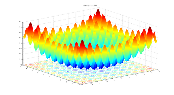
import numpy as np
import math
from geneticalgorithm import geneticalgorithm as ga

def f(X):

    dim=len(X)

    OF=0
    for i in range (0,dim):
        OF+=(X[i]**2)-10*math.cos(2*math.pi*X[i])+10

    return OF


varbound=np.array([[-5.12,5.12]]*2)

model=ga(function=f,dimension=2,variable_type='real',variable_boundaries=varbound)

model.run()

Ackley
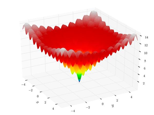
import numpy as np
import math
from geneticalgorithm import geneticalgorithm as ga

def f(X):

    dim=len(X)

    t1=0
    t2=0
    for i in range (0,dim):
        t1+=X[i]**2
        t2+=math.cos(2*math.pi*X[i])

    OF=20+math.e-20*math.exp((t1/dim)*-0.2)-math.exp(t2/dim)

    return OF

varbound=np.array([[-32.768,32.768]]*2)

model=ga(function=f,dimension=2,variable_type='real',variable_boundaries=varbound)

model.run()

Weierstrass
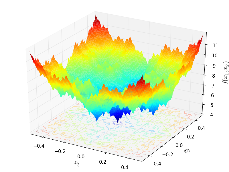
import numpy as np
import math
from geneticalgorithm import geneticalgorithm as ga

def f(X):

    dim=len(X)

    a=0.5
    b=3
    OF=0
    for i in range (0,dim):
        t1=0
        for k in range (0,21):
            t1+=(a**k)*math.cos((2*math.pi*(b**k))*(X[i]+0.5))
        OF+=t1
    t2=0
    for k in range (0,21):
        t2+=(a**k)*math.cos(math.pi*(b**k))
    OF-=dim*t2

    return OF


varbound=np.array([[-0.5,0.5]]*2)

algorithm_param = {'max_num_iteration': 1000,\
                   'population_size':100,\
                   'mutation_probability':0.1,\
                   'elit_ratio': 0.01,\
                   'crossover_probability': 0.5,\
                   'parents_portion': 0.3,\
                   'crossover_type':'uniform',\
                   'max_iteration_without_improv':None}

model=ga(function=f,dimension=2,\
         variable_type='real',\
             variable_boundaries=varbound,
             algorithm_parameters=algorithm_param)

model.run()

License
Copyright 2020 Ryan (Mohammad) Solgi
Permission is hereby granted, free of charge, to any person obtaining a copy of this software and associated documentation files (the "Software"), to deal in the Software without restriction, including without limitation the rights to use, copy, modify, merge, publish, distribute, sublicense, and/or sell copies of the Software, and to permit persons to whom the Software is furnished to do so, subject to the following conditions:
The above copyright notice and this permission notice shall be included in all copies or substantial portions of the Software.
THE SOFTWARE IS PROVIDED "AS IS", WITHOUT WARRANTY OF ANY KIND, EXPRESS OR IMPLIED, INCLUDING BUT NOT LIMITED TO THE WARRANTIES OF MERCHANTABILITY, FITNESS FOR A PARTICULAR PURPOSE AND NONINFRINGEMENT. IN NO EVENT SHALL THE AUTHORS OR COPYRIGHT HOLDERS BE LIABLE FOR ANY CLAIM, DAMAGES OR OTHER LIABILITY, WHETHER IN AN ACTION OF CONTRACT, TORT OR OTHERWISE, ARISING FROM, OUT OF OR IN CONNECTION WITH THE SOFTWARE OR THE USE OR OTHER DEALINGS IN THE SOFTWARE.
Release history Release notifications | RSS feed


Download files
Download the file for your platform. If you're not sure which to choose, learn more about installing packages.
Source Distributions
Built Distribution
Filter files by name, interpreter, ABI, and platform.
If you're not sure about the file name format, learn more about wheel file names.
Copy a direct link to the current filters
File details
Details for the file geneticalgorithm-1.0.2-py3-none-any.whl.
File metadata
- Download URL: geneticalgorithm-1.0.2-py3-none-any.whl
- Upload date:
- Size: 16.1 kB
- Tags: Python 3
- Uploaded using Trusted Publishing? No
- Uploaded via: twine/3.1.1 pkginfo/1.5.0.1 requests/2.22.0 setuptools/51.1.0 requests-toolbelt/0.9.1 tqdm/4.42.1 CPython/3.7.6
File hashes
| Algorithm | Hash digest | |
|---|---|---|
| SHA256 |
24b73642396256d9393ae86902143c14ffdb43ef9345da9d3e888a5e69bc16ae
|
|
| MD5 |
a4e2608661ce440548da9643454c06d3
|
|
| BLAKE2b-256 |
acd2fb9061239eaeee5c0373844f27f43514f33201bc08aea54d65b437402966
|


