
Preference learning with Gaussian processes.



Python implementation of a probabilistic kernel approach to preference learning based on Gaussian processes. Preference relations are captured in a Bayesian framework which allows in turn for global optimization of the inferred functions (Gaussian processes) in as few iterations as possible.
Installation.
Installation
-
From PyPI:
pip install GPro -
From GitHub:
pip install git+https://github.com/chariff/GPro.git
Dependencies
GPro requires:
- Python (>= 3.5)
- NumPy+mkl (>= 1.9.0)
- SciPy (< 1.5.0)
- Pandas (>= 0.24.0)
Brief guide to using GPro.
Checkout the package docstrings for more information.
1. Fitting and making Predictions.
from GPro.preference import ProbitPreferenceGP
import numpy as np
import matplotlib.pyplot as plt
Training data consisting of numeric real positive values. A minimum of two values is required. The following example is in 1D.
X = np.array([2, 1]).reshape(-1, 1)
M is an array containing preferences. A preference is an array of positive integers of shape = (2,). The left integer of a given preference is the index of a value in X which is preferred over another value of X indexed by the right integer of the same preference array. In the following example, 2 is preferred over 1.
M = np.array([0, 1]).reshape(-1, 2)
Instantiate a ProbitPreferenceGP object with default parameters.
gpr = ProbitPreferenceGP()
Fit a Gaussian process. A flat prior with mean zero is applied by default.
gpr.fit(X, M, f_prior=None)
Predict new values.
X_new = np.linspace(-6, 9, 100).reshape(-1, 1)
predicted_values, predicted_deviations = gpr.predict(X_new, return_y_std=True)
Plot.
plt.plot(X_new, np.zeros(100), 'k--', label='GP predictive prior')
plt.plot(X_new, predicted_values, 'r-', label='GP predictive posterior')
plt.plot(X.flat, gpr.predict(X).flat, 'bx', label='Preference')
plt.ylabel('f(X)')
plt.xlabel('X')
# the predicted s.d. is divided for an aesthetic purpose.
plt.gca().fill_between(X_new.flatten(),
                       (predicted_values - predicted_deviations / 50).flatten(),
                       (predicted_values + predicted_deviations / 50).flatten(),
                       color="#b0e0e6", label='GP predictive posterior s.d.')
plt.legend()
plt.show()
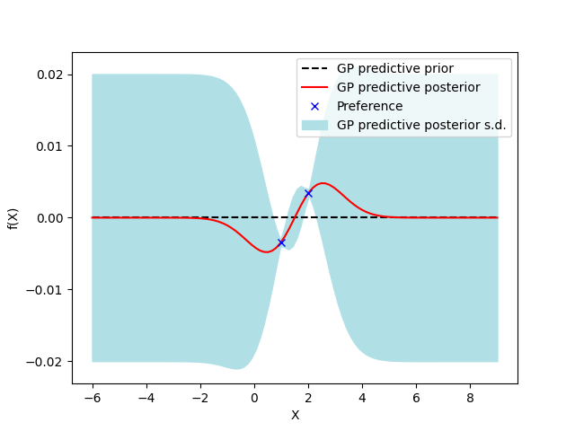
The following plot shows how the posterior predictive Gaussian process is adjusted to the data i.e. 2 is preferred to 1. One can also notice how the standard deviation is small where there is data.
2. Interactive bayesian optimization.
Preference relations are captured in a Bayesian framework which allows for global optimization of the latent function (modelized by Gaussian processes) describing the preference relations. Interactive bayesian optimization with probit responses works by querying the user with a paired comparison and by subsequently updating the Gaussian process model. The iterative procedure optimizes a utility function, seeking a balance between exploration and exploitation of the latent function, to present the user with a new set of instances.
from GPro.kernels import Matern
from GPro.posterior import Laplace
from GPro.acquisitions import UCB
from GPro.optimization import ProbitBayesianOptimization
import numpy as np

# 3D example. Initialization.
X = np.random.sample(size=(2, 3)) * 10
M = np.array([0, 1]).reshape(-1, 2)
Custom parameters for the ProbitBayesianOptimization object. Checkout the package docstrings for more informations on the parameters.
GP_params = {'kernel': Matern(length_scale=1, nu=2.5),
             'post_approx': Laplace(s_eval=1e-5, max_iter=1000,
                                    eta=0.01, tol=1e-3),
             'acquisition': UCB(kappa=2.576),
             'alpha': 1e-5,
             'random_state': None}
Instantiate a ProbitBayesianOptimization object with custom parameters.
gpr_opt = ProbitBayesianOptimization(X, M, GP_params)
Bounded region of optimization space.
bounds = {'x0': (0, 10), 'x1': (0, 10), 'x2': (0, 10)}
Interactive optimization method. Checkout the package docstrings for more informations on the parameters.
console_opt = gpr_opt.interactive_optimization(bounds=bounds, n_init=100, n_solve=10)
optimal_values, suggestion, X_post, M_post, f_post = console_opt
print('optimal values: ', optimal_values)
>>>                   x0        x1        x2
>>> preference  0.306996  3.581879  4.844135
>>> suggestion  0.000000  2.749200  3.287625
>>> Iteration 0, preference (p) or suggestion (s)? (Q to quit): p
>>>                   x0        x1        x2
>>> preference  0.306996  3.581879  4.844135
>>> suggestion  0.289541  4.118421  6.052125
>>> Iteration 1, preference (p) or suggestion (s)? (Q to quit): s
>>>                   x0        x1        x2
>>> preference  0.289541  4.118421  6.052125
>>> suggestion  1.601063  4.300604  5.208000
>>> Iteration 2, preference (p) or suggestion (s)? (Q to quit): Q
>>> optimal values:  [0.28954095 4.11842105 6.05212487]
One can use informative prior. Let's use posterior as prior for the sake of example.
gpr_opt = ProbitBayesianOptimization(X_post, M_post, GP_params)
console_opt = gpr_opt.interactive_optimization(bounds=bounds, n_init=100,
                                               n_solve=10, f_prior=f_post,
                                               max_iter=1, print_suggestion=False)
optimal_values, suggestion, X_post, M_post, f_post = console_opt
print('optimal values: ', optimal_values)
>>>                   x0        x1        x2
>>> preference  0.289541  4.118421  6.052125
>>> suggestion  1.601063  4.300604  5.208000
>>> Iteration 2, preference (p) or suggestion (s)? (Q to quit): Q
>>> optimal values:  [0.28954095 4.11842105 6.05212487]
Download the algorithm with a GUI fully written in python on
2. Bayesian optimization of a black-box function.
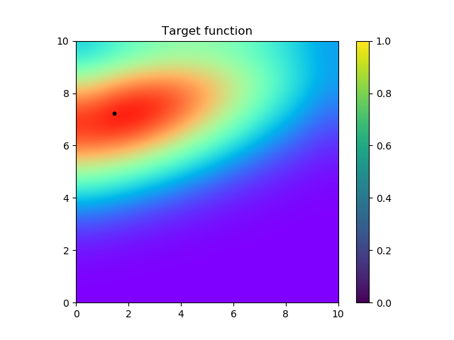
Disclaimer: For testing purposes, we maximize a multivariate normal pdf.
from GPro.kernels import Matern
from GPro.posterior import Laplace
from GPro.acquisitions import UCB
from GPro.optimization import ProbitBayesianOptimization
from scipy.stats import multivariate_normal
import numpy as np
from sklearn import datasets
import matplotlib.cm as cm
import matplotlib.pyplot as plt
Uniform sampling given bounds.
def random_sample(n, d, bounds, random_state=None):
    if random_state is None:
        random_state = np.random.randint(1e6)
    random_state = np.random.RandomState(random_state)
    sample = random_state.uniform(bounds[:, 0], bounds[:, 1],
                                  size=(n, d))
    return sample
Sample parameters of a multivariate normal distribution.
def sample_normal_params(n, d, bounds, scale_sigma=1, random_state=None):
    # sample centroids.
    mu = random_sample(n=n, d=d, bounds=np.array(list(bounds.values())),
                       random_state=random_state)
    # sample covariance matrices.
    sigma = datasets.make_spd_matrix(d, random_state) * scale_sigma
    theta = {'mu': mu, 'sigma': sigma}
    return theta
Example is in 2 dimensions.
d = 2
# Bounded region of optimization space.
bounds = {'x' + str(i): (0, 10) for i in range(0, d)}
# Sample parameters of a d-multivariate normal distribution
theta = sample_normal_params(n=1, d=d, bounds=bounds, scale_sigma=10, random_state=12)
# function to be optimized.
f = lambda x: multivariate_normal.pdf(x, mean=theta['mu'][0], cov=theta['sigma'])
# X, M, init
X = random_sample(n=2, d=d, bounds=np.array(list(bounds.values())))
X = np.asarray(X, dtype='float64')
# Target choices. A preference is an array of positive
# integers of shape = (2,). preference[0], is an index
# of X preferred over preference[1], which is an index of X.
M = sorted(range(len(f(X))), key=lambda k: f(X)[k], reverse=True)
M = np.asarray([M], dtype='int8')
# Parameters for the ProbitBayesianOptimization object.
GP_params = {'kernel': Matern(length_scale=1, nu=2.5),
             'post_approx': Laplace(s_eval=1e-5, max_iter=1000,
                                    eta=0.01, tol=1e-3),
             'acquisition': UCB(kappa=2.576),
             'alpha': 1e-5,
             'random_state': None}
# instantiate a ProbitBayesianOptimization object with custom parameters
gpr_opt = ProbitBayesianOptimization(X, M, GP_params)
Function optimization method.
function_opt = gpr_opt.function_optimization(f=f, bounds=bounds, max_iter=50,
                                             n_init=1000, n_solve=1)

optimal_values, X_post, M_post, f_post = function_opt
print('optimal values: ', optimal_values)
>>> optimal values: [1.45340052 7.22687626]
# rmse
print('rmse: ', .5 * sum(np.sqrt((optimal_values - theta['mu'][0]) ** 2)))
>>> rmse: 0.13092430596422377
# 2d plot
if d == 2:
    resolution = 10
    x_min, x_max = bounds['x0'][0], bounds['x0'][1]
    y_min, y_max = bounds['x1'][0], bounds['x1'][1]
    x = np.linspace(x_min, x_max, resolution)
    y = np.linspace(y_min, y_max, resolution)
    X, Y = np.meshgrid(x, y)
    grid = np.empty((resolution ** 2, 2))
    grid[:, 0] = X.flat
    grid[:, 1] = Y.flat
    Z = f(grid)
    plt.imshow(Z.reshape(-1, resolution), interpolation="bicubic",
               origin="lower", cmap=cm.rainbow, extent=[x_min, x_max, y_min, y_max])
    plt.scatter(optimal_values[0], optimal_values[1], color='black', s=10)
    plt.title('Target function')
    plt.colorbar()
    plt.show()
References:
1 maintainer

Release files for GPro 1.0.5
For a detailed explanation of source distributions (sdists) and built distributions (wheels), please see the package formats documentation.
Source distribution (sdist)
| File | Size | Uploaded | |
|---|---|---|---|
| GPro-1.0.5.tar.gz | 17.3 kB | Details |
Built distribution (wheel)
| File | Interpreter | ABI | Platform | Reset |
|---|---|---|---|---|
| GPro-1.0.5-py3-none-any.whl | Python 3 | none | any | Details |
Total release size: 38.6 kB
Release files / GPro-1.0.5.tar.gz
| Download URL | GPro-1.0.5.tar.gz |
|---|---|
| Size | 17.3 kB |
| Tags | Source |
|
SHA-256 checksum How to use checksums |
34641d0aeb8d3e6fb8cc55d6f73647222f5070b4e9d46afe03debb29f68e4a2f
|
|
BLAKE2b-256 checksum How to use checksums |
1953034ecec0a57059b813f8cf1d915f51162dfdc94945b9f52ccf96f6418946
|
| Upload date | |
|
Uploaded using Trusted Publishing? What is trusted publishing? |
No |
| Uploaded via |
twine/3.3.0 pkginfo/1.6.1 requests/2.25.1 setuptools/50.3.2 requests-toolbelt/0.9.1 tqdm/4.55.0 CPython/3.7.4
|
Release files / GPro-1.0.5-py3-none-any.whl
| Download URL | GPro-1.0.5-py3-none-any.whl |
|---|---|
| Size | 21.3 kB |
| Tags | Python 3 |
|
SHA-256 checksum How to use checksums |
4056e76313101fe4809bf9256f9cb1e9104b361f3c33835da54a76eb414771ed
|
|
BLAKE2b-256 checksum How to use checksums |
56d71c991437a40795b320f58fc0514433c44a9f7c0bee8e3b8c88dc96812be2
|
| Upload date | |
|
Uploaded using Trusted Publishing? What is trusted publishing? |
No |
| Uploaded via |
twine/3.3.0 pkginfo/1.6.1 requests/2.25.1 setuptools/50.3.2 requests-toolbelt/0.9.1 tqdm/4.55.0 CPython/3.7.4
|














