Multi-variable polynomial regression for curve fitting.

Project description
Please reference this package as:
Hampton, J., Tesfalem, H., Fletcher, A., Peyton, A., Brown, M (2021). Reconstructing the conductivity profile of a graphite block using inductance spectroscopy with data-driven techniques. Insight - Non-Destructive Testing and Condition Monitoring, 63(2), 82-87.
Overview
MVPR is available on PyPI, and can be installed via
pip install MVPR
This package fits a multi-variable polynomial equation to a set of data using cross validation. The solution is regularised using truncated singular value decomposition of the Moore-Penrose pseudo-inverse, where the truncation point is found using a golden section search. It is suitable for ill-posed problems, and for preventing over-fitting to noise. Tikohnov regularisation may be included in a future release if there is sufficient demand.
Example
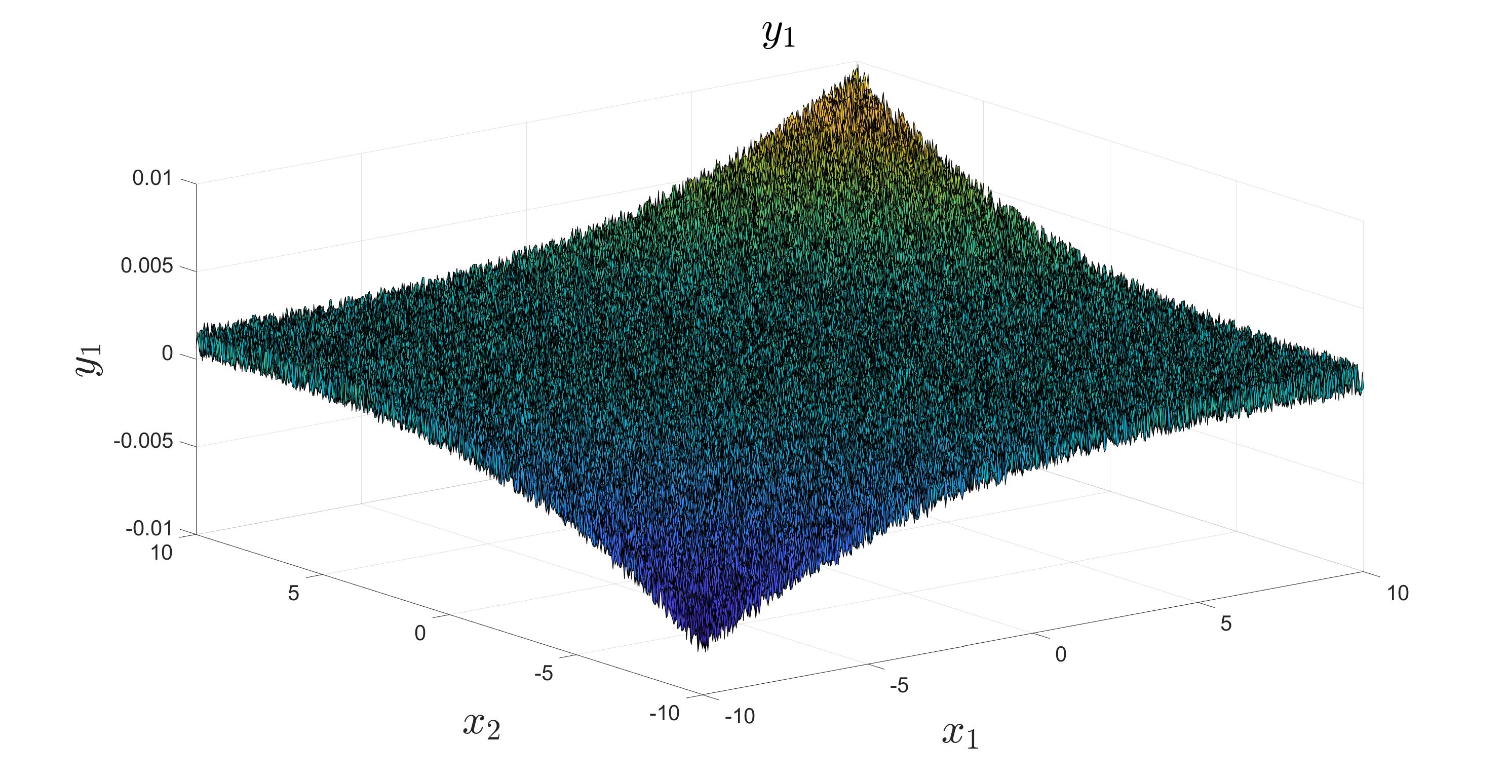
consider a 3-D set of data, plotted as follows:
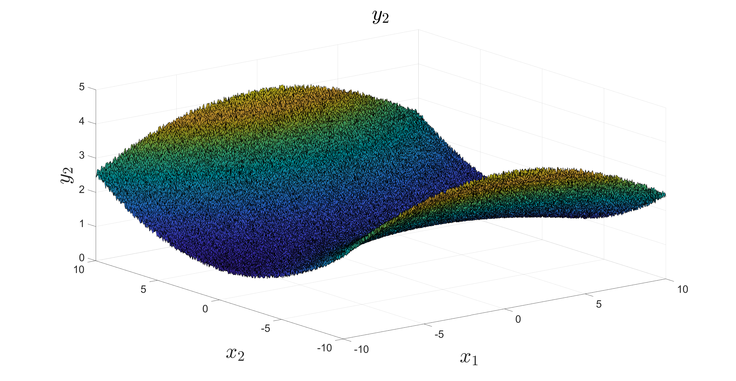
and another set:
We want to find some mapping function for the same input data. Using the MVPR code we can place the vectors into a matrix as (1). This matrix of target data can be split into training, validation or test and passed directly into an MVPR class object. Alternatively, they can be passed seperately into two different instantiations, such that different polynomial orders can be used.

First import the data:
import MVPR as MVP
import numpy as np
import pandas as pd
from openpyxl import load_workbook
df= pd.read_excel(r'C:\Users\filepath\data.xlsx')
data=df.to_numpy()
df= pd.read_excel(r'C:\Users\filepath\targets.xlsx')
targets=df.to_numpy()
select the proportions of data for cross-validation
proportion_training = 0.9
num_train_samples = round(len(data[:,0])*proportion_training)
num_val_samples = round(len(data[:,0]))-num_train_samples
standardise:
mean_dat = data[:, :].mean(axis=0)
std_dat = data[:, :].std(axis=0)

data -= mean_dat

if 0 not in std_dat:
    data[:, :] /= std_dat

training_data = data[:num_train_samples, :]
training_targets = targets[:num_train_samples, :]

validation_data = data[-num_val_samples :, :]
validation_targets = targets[-num_val_samples :, :]
call the following
M = MVP.MVPR_forward(training_data, training_targets, validation_data, validation_targets)

optimum_order = M.find_order()
coefficient_matrix = M.compute_CM(optimum_order)

predicted_validation = M.compute(coefficient_matrix, optimum_order, validation_data)

df = pd.DataFrame(predicted_validation)
df.to_excel(r'C:\Users\filepath\predicted.xlsx')
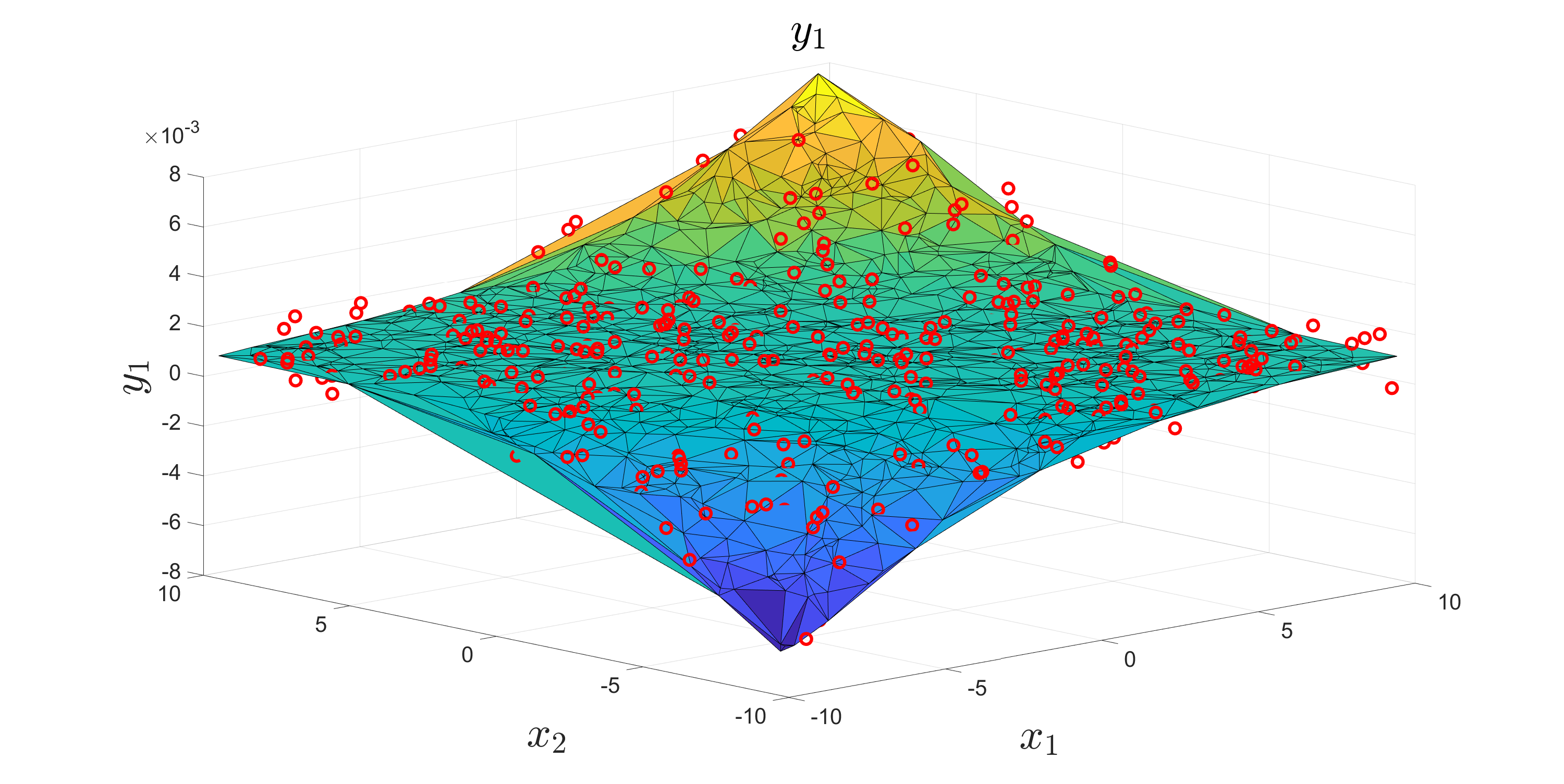
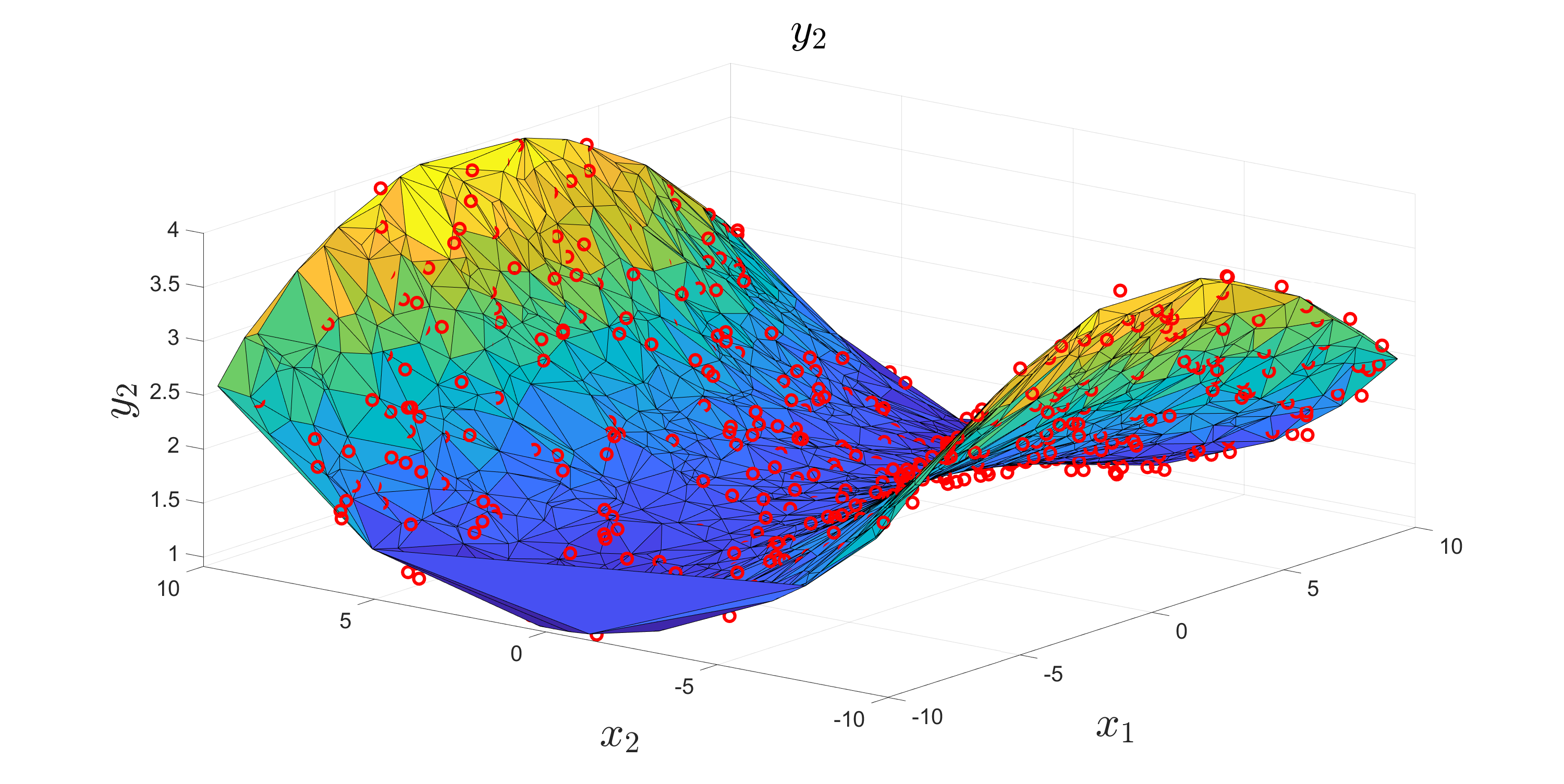
The fitted curves:
Functions and arguments
import MVPR as MVP
:
MVPR_object = MVP.MVPR_forward(training_data, training_targets, validation_data, validation_targets, verbose=True, search = 'exponent')
The verbose argument is optional, its default value is false.
The truncation point can either be written as 10^a or as b, the input argument 'search' specifies whether we search for the value of a or b; see the following code segment from the golden section search:
:
if self.search == 'exponent':
   distance = 0.61803398875 * (np.log10(ind_high_1) - np.log10(ind_low_1))
   ind_low_2 = round(10 ** (np.log10(ind_high_1) - distance))
   ind_high_2 = round(10 ** (np.log10(ind_low_1) + distance))
else:
   distance = 0.61803398875 * (ind_high_1 - ind_low_1)
   ind_low_2 = round(ind_high_1 - distance)
   ind_high_2 = round(ind_low_1 + distance)
:
optimal_order=MVPR_object.find_order()
This function finds the optimal order of polynomial in the range 0 to 6, using cross validation.
MVPR_object.compute_CM(order)
This function computes the coefficient matrix which fits a polynomial to the measured data in a least squares sense. The fit is regularised using truncated singular value decomposition, which eliminates singular values under a certain threshold. Any oder can be passed into this by the user, it does not have to have the range limited in find_oder().
Theory
For the theory behind the code see [1] and [2].
References
[1] Hansen, P. C. (1997). Rank-deficient and Discrete Ill-posed Problems: Numerical Aspects of Linear Inversion.
[2] Hampton, J., Tesfalem, H., Fletcher, A., Peyton, A., Brown, M (2021). Reconstructing the conductivity profile of a graphite block using inductance spectroscopy with data-driven techniques. Insight - Non-Destructive Testing and Condition Monitoring, 63(2), 82-87.
Release history Release notifications | RSS feed


Download files
Download the file for your platform. If you're not sure which to choose, learn more about installing packages.
Source Distribution
Built Distribution
Filter files by name, interpreter, ABI, and platform.
If you're not sure about the file name format, learn more about wheel file names.
Copy a direct link to the current filters
File details
Details for the file MVPR-1.32.tar.gz.
File metadata
- Download URL: MVPR-1.32.tar.gz
- Upload date:
- Size: 6.9 kB
- Tags: Source
- Uploaded using Trusted Publishing? No
- Uploaded via: twine/3.4.2 importlib_metadata/4.8.1 pkginfo/1.7.1 requests/2.25.1 requests-toolbelt/0.9.1 tqdm/4.62.2 CPython/3.8.8
File hashes
| Algorithm | Hash digest | |
|---|---|---|
| SHA256 |
b797b7da4fe087f517b17480addb66b46323c736c9983c95fec0efba9b5c5fc1
|
|
| MD5 |
407c9f44ee1f98923204c46d2c8b95cd
|
|
| BLAKE2b-256 |
d3548dc6c69cb1841d2cfe774e6522224bdeb1c820db642612ecd59b7be3dd8a
|
File details
Details for the file MVPR-1.32-py3-none-any.whl.
File metadata
- Download URL: MVPR-1.32-py3-none-any.whl
- Upload date:
- Size: 6.9 kB
- Tags: Python 3
- Uploaded using Trusted Publishing? No
- Uploaded via: twine/3.4.2 importlib_metadata/4.8.1 pkginfo/1.7.1 requests/2.25.1 requests-toolbelt/0.9.1 tqdm/4.62.2 CPython/3.8.8
File hashes
| Algorithm | Hash digest | |
|---|---|---|
| SHA256 |
c9d0913e00b94be52c4df5343415272a6138611ff9403865b9227ab0bdb3c584
|
|
| MD5 |
4119dbb02de722bc43cd15622ed2ac8e
|
|
| BLAKE2b-256 |
6f9da931de655a33ff0cb9cc57bcaed98b8f7480f9cd027109d2a4a7d58d886d
|


