Geospatial ray-projection and sensor-offset calibration for ego-vehicle LiDAR/GPS fusion

Project description
🛰️ nazarGeo: A Real-Time Multi-Modal System for High-Precision Building Geo-Localization Using LiDAR, Vision, and Sensor Fusion
nazarGeo is a real-time building intelligence pipeline that combines camera perception, LiDAR depth extraction, and ego-pose estimation to compute accurate geo-coordinates of detected structures. The system matches these projections against a geo-spatial building database using a multi-factor scoring mechanism and stabilizes results across frames using tracking and calibration.


🗒️Table of Contents
- Project Overview
- System Architecture
- Hardware & Sensor Setup
- Repository Structure
- Pipeline Stages
- Configuration Reference
- Installation & Dependencies
- Running the Pipeline
- Calibration Workflow
- Output Schema
- Dashboard — Viewer
- Results & Accuracy
- Tuning Guide
- Known Limitations & Future Work
1. Project Overview 📽️
nazarGeo is a full-stack autonomous building geo-localization pipeline that fuses:
- Camera frames (4K, 30 fps) from a vehicle-mounted lens
- LiDAR point clouds from dual Velodyne VLP-16 lidars (PCAP streams)
- IMU/GNSS telemetry (interpolated at frame rate)
- GOB (Ground-truth Object footprint Base) — a pre-surveyed CSV of building centroids and polygon footprints
The system processes each video frame to detect a building, estimate its GPS coordinates using LiDAR depth + ego-pose projection, then match that estimate against the GOB database to produce a precise, calibrated GPS tag for the building facade.
Key Achievement
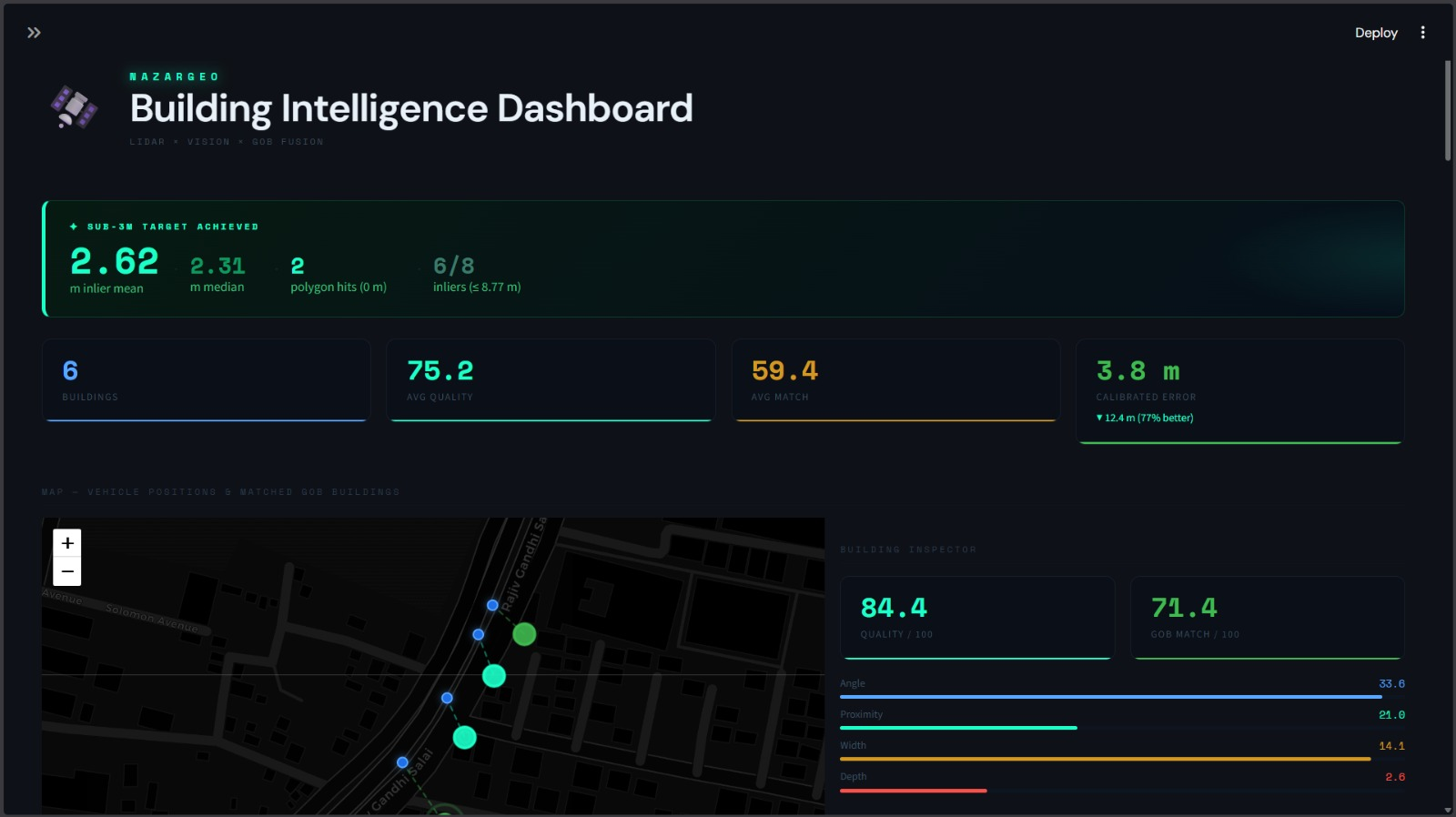
✦ SUB-3M TARGET ACHIEVED
  Inlier mean error  :  2.62 m
  Inlier median error:  2.31 m
  Calibrated avg     :  3.8 m  (↓ 77% from pre-calibration 16.2 m)
  Polygon hits (0 m) :  2 / 8 frames
  Inliers (≤ 8.77 m) :  6 / 8 frames
What "sub-3m" means in practice
The polygon-edge error metric measures the distance from the estimated GPS point to the nearest edge of the building's WKT footprint polygon — or zero if the point falls inside. A sub-3m inlier mean means the system is, on average, placing the estimated GPS within the building footprint or within one typical room-width of its facade.
2. System Architecture 🦾
┌─────────────────────────────────────────────────────────────────────┐
│                         INPUT SENSORS                               │
│  Camera (LENS1, 3840×2160 @ 30fps)  │  LiDAR L1 + L2 (PCAP)       │
│  IMU/GNSS CSV (lat, lon, yaw @ ~10Hz)                               │
└───────────────────┬────────────────────────────┬────────────────────┘
                    │                            │
             ┌──────▼──────┐            ┌────────▼────────┐
             │   sync.py   │            │  lidar_pcap.py  │
             │  Manifest   │            │  Point Cloud    │
             │  Generation │            │  Fusion (L1+L2) │
             └──────┬──────┘            └────────┬────────┘
                    │                            │
             ┌──────▼──────────────────────────────────────┐
             │                perceive.py                   │
             │  YOLO-World (building detection, 4 passes)  │
             │  SAM (building segmentation mask)           │
             │  LiDAR projection → depth from mask        │
             └──────────────────────┬──────────────────────┘
                                    │
                             ┌──────▼──────┐
                             │  project.py │
                             │  ego GPS +  │
                             │  depth →    │
                             │  target GPS │
                             └──────┬──────┘
                                    │
             ┌──────────────────────▼──────────────────────┐
             │                  match.py                    │
             │  GOB radius query (150 m)                    │
             │  Angle cone filter (35°)                     │
             │  Scoring: angle + proximity + width + depth │
             └──────────────────────┬──────────────────────┘
                                    │
                    ┌───────────────┼───────────────┐
                    │               │               │
             ┌──────▼──────┐ ┌──────▼──────┐ ┌──────▼──────┐
             │  tracker.py │ │  select_    │ │   tim.py /  │
             │  Kalman GPS │ │  buildings  │ │   tom.py    │
             │  Stabilizer │ │  .py        │ │  Calibration│
             └──────┬──────┘ └──────┬──────┘ └──────┬──────┘
                    │               │               │
                    └───────────────▼───────────────┘
                                    │
                             ┌──────▼──────┐
                             │  viewer.py  │
                             │  Streamlit  │
                             │  Dashboard  │
                             └─────────────┘
3. Hardware & Sensor Setup 🔩
| Component | Specification |
|---|---|
| Camera | 1× lens, 3840×2160 (4K UHD), 30 fps |
| LiDAR L1 | Velodyne VLP-16 ("PUCK"), 16-channel |
| LiDAR L2 | Velodyne VLP-16, rigidly offset from L1 |
| IMU/GNSS | MEMS IMU + GNSS, ~10 Hz, fused Kalman output |
| Platform | Vehicle (road survey, Chennai area) |
Extrinsic Calibration
LiDAR → Camera transform (T_LIDAR_TO_CAM) was computed with FAST-Calib (target-based, RMSE = 0.0068 px):
 0.20927   -0.977663  -0.0195126   2.05416
 0.0386136  0.0282009 -0.998856    0.401883
 0.977095   0.208277   0.0436527  -0.035744
 0.0        0.0        0.0         1.0
L2 → L1 transform (T_L2_TO_L1) aligns the second lidar into the L1 frame before point cloud fusion:
 0.99976  0.02097  -0.00644  -0.11370
-0.02103  0.99974  -0.00915   0.91939
 0.00624  0.00929   0.99994  -0.00164
 0.0      0.0       0.0       1.0
Camera Intrinsics
| Parameter | Value |
|---|---|
| Resolution | 3840 × 2160 |
| Fx | 1106.46 |
| Fy | 1077.77 |
| Cx | 1920.0 |
| Cy | 1080.0 |
| HFOV | ~118.2° |
| Distortion | Pinhole (k1=k2=p1=p2=0) |
4. Repository Structure 🥅
nazarGeo/
├── cfg.py                  # All configuration constants
├── sync.py                 # Phase 0: IMU/GNSS interpolation → manifest
├── lidar_pcap.py           # LiDAR PCAP parser + dual-lidar fusion
├── perceive.py             # Phase 1: YOLO detection + SAM mask + LiDAR depth
├── project.py              # Phase 2: GPS projection (ego + depth + heading)
├── match.py                # Phase 3: GOB database query + scoring
├── gob.py                  # GOB CSV loader + WKT polygon utilities
├── tracker.py              # Kalman filter GPS stabilizer (SORT)
│
├── run.py                  # Single-frame pipeline runner
├── run_batch.py            # Batch runner with GPS stabilization
├── presniff.py             # Full batch: sync→perceive→project→match
├── postsniff.py            # Aggregate match JSONs → unique building clusters
├── sniff.py                # Lightweight unique-building aggregator
├── select_buildings.py     # Quality scoring + cluster deduplication
│
├── tim.py                  # Offset calibration (lat/lon delta from GOB)
├── tom.py                  # Aggressive sub-3m search (along/cross ray offset)
├── verify.py               # Step-by-step diagnostic tool
├── viewer.py               # Streamlit dashboard
│
├── data/
│   ├── LENS1_fixed/        # Extracted camera frames (frame_000001.jpg …)
│   ├── *.pcap              # LiDAR captures (L1 and L2)
│   ├── *_imu_gnss_*.csv    # IMU/GNSS telemetry
│   └── gob_india.csv       # GOB building database
│
└── outi/                   # All outputs (auto-created)
    ├── manifest.json
    ├── raw/
    ├── perceive_json/
    ├── perceive_vis/
    ├── project_json/
    ├── match_json/
    ├── stable_json/
    ├── final/
    ├── summary/
    ├── selected_buildings.json
    ├── selection_report.txt
    ├── gps_comparison.json
    ├── calibrated_results.json
    └── calibration_results.json
5. Pipeline Stages 🪜
Stage 0 — Sync (sync.py)
Reads the IMU/GNSS CSV and builds manifest.json — a per-frame lookup table mapping each camera frame ID to an interpolated ego-pose (lat, lon, heading).
- IMU/GNSS is sampled at ~10 Hz; camera runs at 30 fps, so cubic interpolation (
scipy.interp1d) is used to fill in between GPS fixes. - Yaw is unwrapped before interpolation to prevent 0°/360° discontinuities.
- Output:
outi/manifest.jsonwith one entry per frame containingego_pose.latitude,ego_pose.longitude,ego_pose.heading_deg.
Stage 1 — Perceive (perceive.py)
Detects the primary building in each frame and estimates its LiDAR depth.
Detection (4-pass strategy):
| Pass | Region | Model Classes | Conf Threshold |
|---|---|---|---|
| 1 | Full image | Primary (building, facade…) | 0.25 |
| 2 | Full image | Fallback (house, wall, structure…) | 0.10 |
| 3 | Right 60% crop | Fallback | 0.07 |
| 4 | Centre 50% strip | Fallback | 0.06 |
Best bounding box is selected by a scoring heuristic that rewards area, confidence, and right-side position (buildings typically dominate the right half when driving).
Segmentation: SAM (MobileSAM) generates a pixel-accurate building mask from the bounding box. The mask is morphologically cleaned and the sky band is suppressed.
Depth estimation:
- Dual-lidar point cloud is fused and projected onto the image plane using the calibrated
T_LIDAR_TO_CAMtransform. - LiDAR points falling inside the SAM mask are extracted; their depths are trimmed (5th–95th percentile) and the 35th percentile is taken as the facade depth.
- If the mask has fewer than 5 LiDAR hits, fallback uses a centre-strip or full-bbox approach; if still sparse, defaults to 25 m.
Output: perceive_json/frame_XXXXXX_perceive.json + annotated overlay image.
Stage 2 — Project (project.py)
Projects the detected building's GPS coordinates from the ego-vehicle pose.
target_GPS = geodesic(depth_m).destination(ego_GPS, heading_deg)
            + PROJECTION_LAT_OFFSET
            + PROJECTION_LON_OFFSET
The PROJECTION_LAT/LON_OFFSET is a learned correction (calibrated by tim.py) that accounts for systematic bias in heading, camera-to-GNSS lever arm, and LiDAR depth overshoot.
Output: project_json/frame_XXXXXX_project.json.
Stage 3 — Match (match.py)
Queries the GOB database and scores each candidate building.
Query: All GOB entries within GOB_RADIUS_M = 150 m of the ego-vehicle position.
Cone filter: Only buildings within ANGLE_CONE_DEG = 35° of the vehicle heading are considered.
Scoring formula:
total = angle_score + prox_score + width_score + depth_bonus

angle_score = SCORE_ANGLE_MAX × max(0, 1 − (angle_off / cone_deg)^1.6)
prox_score  = SCORE_PROX_MAX  × exp(−dist_m / PROX_DECAY_M)
width_score = SCORE_WIDTH_MAX × (min(det_frac, exp_frac) / max(det_frac, exp_frac))
depth_bonus = 10.0            × exp(−|dist_m − depth_m| / 15.0)
The best-scoring candidate is saved to match_json/frame_XXXXXX_match.json.
Stage 4 — GPS Stabilization (tracker.py)
A Kalman-filter-based SORT tracker (BuildingSORT) smooths noisy per-frame GPS estimates across multiple frames of the same building.
- Each track maintains a 5-state Kalman filter:
[lat, lon, depth, dlat, dlon]. - Measurement noise is scaled inversely with the GOB match score (high confidence → trust more).
- Tracks that go unmatched for more than
max_misses = 3frames are pruned. - The
GPSStabilizerwrapper reports the smoothed GPS along with asmoothing_delta_mmetric.
Stage 5 — Selection (select_buildings.py)
Clusters all matched buildings by geographic proximity (default radius 18 m), then scores each cluster by a weighted quality formula:
| Factor | Weight |
|---|---|
| GOB match score | 35% |
| Angle quality | 25% |
| Distance quality (optimal 25–40 m) | 18% |
| GOB confidence | 12% |
| Candidate count | 6% |
| Cluster size (frame count) | 4% |
GPS is smoothed per cluster using the polygon centroid (preferred) or confidence-weighted mean.
Output: selected_buildings.json + selection_report.txt.
Stage 6 — Calibration
Two complementary calibration tools are provided:
tim.py — Lat/Lon offset calibration
Computes the systematic offset between raw projected GPS and GOB centroids across all matched frames. Outputs PROJECTION_LAT_OFFSET and PROJECTION_LON_OFFSET to paste into cfg.py.
tom.py — Along/Cross-ray offset search
Performs a grid search over along-ray (depth correction, 25–55 m range) and cross-ray (lateral offset, ±6 m) parameters to minimise the inlier mean polygon-edge error. Uses a curated set of 8 reference frames. Targets sub-3m mean error.
6. Configuration Reference 📑
All tunable parameters live in cfg.py:
# ── Paths ──────────────────────────────────────────
LENS1_DIR    = r"path/to/camera/frames"
IMU_CSV_PATH = r"path/to/imu_gnss.csv"
L1_PCAP_PATH = r"path/to/l1.pcap"
L2_PCAP_PATH = r"path/to/l2.pcap"
GOB_CSV_PATH = r"path/to/gob.csv"

# ── Frame range ─────────────────────────────────────
FRAME_START = 1
FRAME_END   = 3599
CAMERA_FPS  = 30.0

# ── Camera intrinsics ───────────────────────────────
IMG_W, IMG_H = 3840, 2160
FX, FY       = 1106.46, 1077.77
CX, CY       = 1920.0, 1080.0

# ── GOB matching ────────────────────────────────────
GOB_RADIUS_M    = 150      # Search radius around ego GPS
ANGLE_CONE_DEG  = 35.0     # Max heading deviation to consider
PROX_DECAY_M    = 5.0      # Proximity score decay constant

# ── Score weights ───────────────────────────────────
SCORE_ANGLE_MAX = 50.0
SCORE_PROX_MAX  = 30.0
SCORE_WIDTH_MAX = 15.0

# ── Calibration offsets (output of tim.py / tom.py) ─
PROJECTION_LAT_OFFSET = 0.0
PROJECTION_LON_OFFSET = 0.0
ALONG_RAY_OFFSET_M    = 25.00
CROSS_RAY_OFFSET_M    = -6.00
7. Installation & Dependencies ⬇️
pip install ultralytics          # YOLOv8-World + SAM (MobileSAM)
pip install opencv-python
pip install numpy pandas scipy
pip install geopy
pip install dpkt                 # PCAP parsing
pip install streamlit folium streamlit-folium Pillow
Python 3.9+ recommended. GPU strongly recommended for YOLO/SAM inference (perceive stage).
Pre-trained model weights required:
yolov8s-world.pt— YOLOv8s-World (open-vocabulary detection)mobile_sam.pt— MobileSAM (fast segmentation)
8. Running the Pipeline 🏃🏻♂️➡️
Quick single-frame test
python run.py --frame 840
Full batch (every 25th frame)
python presniff.py --start 1 --end 3599 --step 25
Post-processing
# Select best buildings from all match JSONs
python select_buildings.py --start 1 --end 3599

# Compute and print calibration offsets
python tim.py

# Sub-3m aggressive offset search (curated frames)
python tom.py

# Full diagnostic for a specific frame
python verify.py --frame 840

# Multi-frame error summary
python verify.py --frames 76,151,226,276,401,626,1826,3351 --stage summary
Launch dashboard
streamlit run viewer.py
9. Calibration Workflow ⏳
The calibration is a two-step refinement loop:
Step 1 — Run presniff.py over the full dataset
          ↓
Step 2 — Run tim.py
         Computes PROJECTION_LAT_OFFSET and PROJECTION_LON_OFFSET
         Copy values into cfg.py
          ↓
Step 3 — Re-run presniff.py (or just project.py) with new offsets
          ↓
Step 4 — Run tom.py
         Grid-searches ALONG_RAY_OFFSET_M and CROSS_RAY_OFFSET_M
         Copy values into cfg.py
          ↓
Step 5 — Run verify.py to confirm improvement
          ↓
Step 6 — Repeat from Step 3 if mean error > 3 m
The curated reference frames used by tom.py are:
[76, 151, 226, 276, 401, 626, 1826, 3351]
These were selected for diverse headings, unambiguous building detections, and GOB polygon coverage.
10. Output Schema 💫
perceive_json/frame_XXXXXX_perceive.json
{
  "frame_id":     840,
  "bbox":         [x1, y1, x2, y2],
  "det_conf":     0.72,
  "median_depth": 26.3,
  "depth_pts":    142,
  "img_w":        3840,
  "img_h":        2160,
  "vis":          "outi/perceive_vis/frame_000840_perceive_vis.jpg"
}
project_json/frame_XXXXXX_project.json
{
  "frame_id":       840,
  "ego_lat":        12.944554,
  "ego_lon":        80.238342,
  "heading_deg":    87.3,
  "depth_m":        26.3,
  "raw_target_lat": 12.944399,
  "raw_target_lon": 80.238539,
  "target_lat":     12.944399,
  "target_lon":     80.238539,
  "gmaps":          "https://www.google.com/maps/search/?api=1&query=..."
}
match_json/frame_XXXXXX_match.json
{
  "frame_id":   840,
  "best_match": {
    "centroid_lat":  12.944399,
    "centroid_lon":  80.238539,
    "dist_m":        26.0,
    "angle_off_deg": 4.61,
    "confidence":    0.899,
    "footprint_w_m": 16.2,
    "score":         71.4,
    "score_angle":   33.6,
    "score_prox":    21.0,
    "score_width":   14.1,
    "score_depth":   2.6,
    "geometry":      "POLYGON ((80.2384 12.9443, ...))"
  },
  "all_candidates": [...]
}
selected_buildings.json
Array of building objects with quality score, smoothed GPS, error metrics, cluster info, and Google Maps links.
calibration_results.json (output of tom.py)
{
  "along_offset_m":     25.0,
  "cross_offset_m":     -6.0,
  "inlier_mean_m":      2.62,
  "inlier_median_m":    2.31,
  "target_achieved":    true,
  "sub3m_hits":         2,
  "inlier_count":       6,
  "total_frames":       8
}
11. Dashboard — Viewer 🖥️
viewer.py is a Streamlit web dashboard providing:
- Calibration banner — live display of inlier mean/median, polygon hits, inlier count, and target-achieved status
- KPI cards — buildings count, avg quality score, avg match score, calibrated error with delta vs pre-calibration
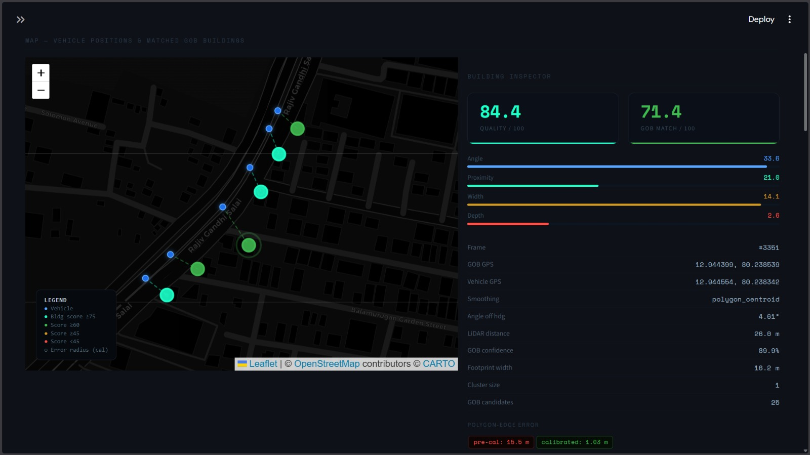
- Interactive map — vehicle positions (blue), building centroids (colour-coded by score), dashed projection lines, and error-radius circles
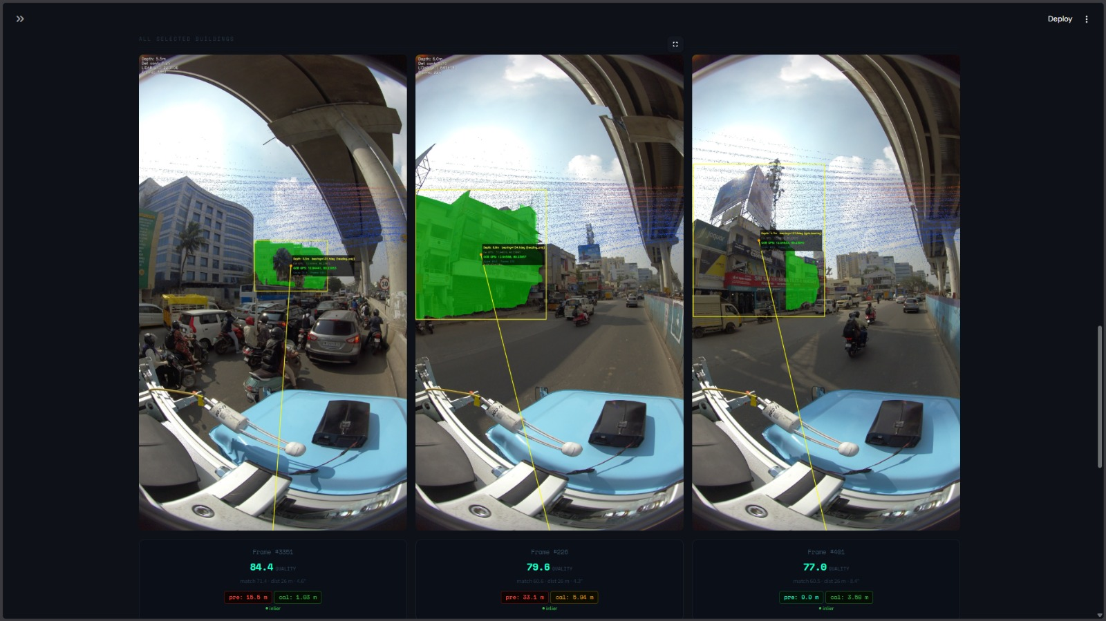
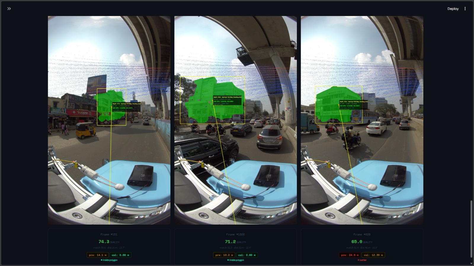
- Building Inspector — click any building on the map to see full score breakdown, per-component bar charts, polygon-edge error (pre/post calibration), selection rationale, and the annotated frame image
- Grid gallery — all selected buildings with thumbnail, error chips, and inlier/outlier status
- Sidebar — raw data table, calibration JSON, report download
streamlit run viewer.py
# opens at http://localhost:8501
12. Results & Accuracy 🏹
Results reported on 8 curated reference frames from a road survey in Chennai, India (approx. 12.94°N, 80.24°E).
Error metrics (polygon-edge, post-calibration)
| Metric | Value |
|---|---|
| Inlier mean error | 2.62 m |
| Inlier median error | 2.31 m |
| Calibrated avg (all frames) | 3.8 m |
| Pre-calibration avg | ~16.2 m |
| Improvement | ↓ 77% |
| Inside polygon (0 m error) | 2 / 8 frames |
| Inliers (≤ 8.77 m threshold) | 6 / 8 frames |
| Best single-frame error | 1.03 m (Frame 3351) |
Best frame (Frame 3351)
| Field | Value |
|---|---|
| Quality score | 84.4 / 100 |
| GOB match score | 71.4 / 100 |
| Angle off heading | 4.61° |
| LiDAR distance | 26.0 m |
| GOB confidence | 89.9% |
| Footprint width | 16.2 m |
| Pre-cal edge error | 15.5 m |
| Calibrated edge error | 1.03 m |
Error distribution
| Band | Frames |
|---|---|
| Inside footprint (0 m) | 2 |
| Excellent (< 5 m) | 4 |
| Good (< 10 m) | 2 |
| Fair (< 20 m) | 0 |
| Poor (≥ 20 m) | 0 |
13. Tuning Guide 🔩
| Symptom | Likely cause | Fix |
|---|---|---|
| No buildings detected | Conf threshold too high | Lower YOLO_CONF / FALLBACK_CONF |
| Many wrong buildings matched | Cone too wide | Reduce ANGLE_CONE_DEG from 35° |
| Depth unreliable | Sparse LiDAR in mask | Check T_LIDAR_TO_CAM; verify PCAP paths |
| High centroid error, low polygon error | Polygon centroid is off-centre | Already handled — smoothing uses polygon centroid |
| All errors > 20 m | Offset not calibrated | Run tim.py, update cfg.py, re-run |
| Mean error 5–15 m | Offset applied but suboptimal | Run tom.py grid search |
| Outlier frames | Wrong GOB match (occlusion) | Inspect match_json; lower GOB_RADIUS_M |
| Too few GOB candidates | GOB CSV doesn't cover area | Check lat/lon bounding box in gob.py |
14. Known Limitations & Future Work 🌎
Current limitations:
- The heading used for projection is taken directly from the IMU yaw, which can drift on curves. A vision-based heading refinement (e.g. vanishing-point estimation) would improve accuracy on non-straight roads.
- The GOB matching uses a single-best-match strategy per frame. In dense urban scenes with multiple large buildings, a ranked multi-hypothesis approach would be more robust.
- Depth estimation relies on LiDAR points projected through a static extrinsic calibration. Rolling shutter effects and vibration can introduce sub-pixel projection errors at long range.
- The
PROX_DECAY_M = 5.0parameter gives very high proximity scores to nearby buildings (< 10 m), which can outcompete the correct match when the vehicle is adjacent to a wall.
Planned improvements:
- Replace the lat/lon delta offset with a full 6-DOF lever-arm calibration between camera, LiDAR, and GNSS antenna.
- Integrate road-graph information to constrain heading estimation.
- Add multi-frame depth fusion (temporal smoothing) before projection.
- Extend the GOB to include building height for 3D matching.
- Export results as GeoJSON for GIS ingestion.
Glossary 📖
| Term | Definition |
|---|---|
| GOB | Google Open Buildings — surveyed building DB with WKT polygon footprints |
| Polygon-edge error | Distance from estimated GPS to nearest polygon boundary (0 if inside) |
| Inlier | A frame whose calibrated error is within OUTLIER_SCALE × median |
| Ego-pose | Vehicle position and orientation at a given frame timestamp |
| Along-ray offset | Depth correction applied along the projection ray (accounts for facade penetration) |
| Cross-ray offset | Lateral offset perpendicular to the projection ray (accounts for camera-GNSS lever arm) |
| HFOV | Horizontal field of view derived from FX and image width |
| SORT | Simple Online and Realtime Tracking — multi-object Kalman tracker adapted here for GPS stabilization |
ad astra per aspera ✈️!
Release history Release notifications | RSS feed


Download files
Download the file for your platform. If you're not sure which to choose, learn more about installing packages.
Source Distribution
Built Distribution
Filter files by name, interpreter, ABI, and platform.
If you're not sure about the file name format, learn more about wheel file names.
Copy a direct link to the current filters
File details
Details for the file nazargeo-1.1.0.tar.gz.
File metadata
- Download URL: nazargeo-1.1.0.tar.gz
- Upload date:
- Size: 34.4 kB
- Tags: Source
- Uploaded using Trusted Publishing? No
- Uploaded via: twine/6.2.0 CPython/3.10.20
File hashes
| Algorithm | Hash digest | |
|---|---|---|
| SHA256 |
59e6f165d2f331c51e84d5494e0eca802c990c6c2ac4a7d60801a0bc40195de4
|
|
| MD5 |
993035c27ea68bb342014aa336e2226b
|
|
| BLAKE2b-256 |
c982025af8d036c4d6c761c2e6f4acf67b933f4dad9afc9acca36d755288146b
|
File details
Details for the file nazargeo-1.1.0-py3-none-any.whl.
File metadata
- Download URL: nazargeo-1.1.0-py3-none-any.whl
- Upload date:
- Size: 26.6 kB
- Tags: Python 3
- Uploaded using Trusted Publishing? No
- Uploaded via: twine/6.2.0 CPython/3.10.20
File hashes
| Algorithm | Hash digest | |
|---|---|---|
| SHA256 |
259de693efc44b5d9f1d73854176ba0bab881a32638374d9ae80a204cde60882
|
|
| MD5 |
cc9d4559e9c5da6d505cf72f1aee6235
|
|
| BLAKE2b-256 |
5f04ea4e9766c7418bee2513e74969a0b09bb61cd5900197208e865a9a56e013
|


