
This release is a pre-release and may not be stable for production use.
OptiKit

Summary
This Python module provides a comprehensive suite of tools for studying and applying optics principles, particularly focusing on wave optics. The module is designed to generate families of solutions to the paraxial wave equation, which is fundamental in understanding the behavior of light in optical systems. Additionally, it includes functionalities for hologram generation, light propagation, and analysis of Stokes parameters, which describe the polarization state of light. These tools are essential for research and applications in optical engineering, laser physics, and related fields.
Solutions to the paraxial wave equation in various coordinate systems.
- Hermite-Gaussian Modes in cartesian coordinates
- Laguerre-Gaussian Modes in cylindrical coordinates
- Ince-Gaussian Modes in elyptical coordinates
Library installation
Requirements
- numpy
- pillow
- scipy
- matplotlib
- python >= 3.10
pip install optikit
Gaussian Modes
$U(r, \theta, z) = \frac{\omega_0}{\omega(z)}\exp{\frac{-r^2}{\omega(z)^2}} \exp{\left(-i\left(kz + k\frac{r^2}{2R(z)} - \Psi(z) \right)\right)}$
where r is the radius, $\omega_0$ represents the beam width at $z = 0$, $\omega(z) = \omega_0\sqrt{1 + z^2/z_R^2}$ describes the beam width, $R(z) = z + z^2_R/z$ is the radius of curvature of the phase front, $z_R = k\omega_0^2/2$ is the Rayleigh range and $\Psi = arctan(z/z_R)$ is the Gouy shift.
Code implementation
from optikit.Beam import Beam

Gauss = Beam(type = 'Gaussian',
            size = 5e-3, # in meters
            shape = 501, # Number of points
            w0 = 1e-3, # Beam width
            k = (2*np.pi/632.8e-9), # wavenumber
            z = 0)
Gauss.plot_amplitude()
Ince-Gaussian Modes
The Ince-Gaussian (IG) mode is a solution to the paraxial wave equation expressed in elliptic coordinates $(\xi, \eta)$. The general form of an Ince-Gaussian beam $(\xi, \eta, z)$ can be written as:
$\text{IG}_{p,m}^e(\mathbf{r}, \epsilon) = \frac{C\omega_0}{\omega(z)}C_p^m(i\xi, \epsilon)C_p^m(\eta, \epsilon)\exp\left[\frac{-r^2}{\omega^2(z)}\right] \exp\left(i\left[kz + \frac{kr^2}{2R(z)} - (p - 1) \Psi(z)\right]\right)$,
$\text{IG}_{p,m}^o(\mathbf{r}, \epsilon) = \frac{S\omega_0}{\omega(z)}S_p^m(i\xi, \epsilon)S_p^m(\eta, \epsilon)\exp\left[\frac{-r^2}{\omega^2(z)}\right] \exp\left(i\left[kz + \frac{kr^2}{2R(z)} - (p - 1) \Psi(z)\right]\right)$
where r is the radius, $\omega_0$ represents the beam width at $z = 0$, $\omega(z) = \omega_0\sqrt{1 + z^2/z_R^2}$ describes the beam width, $R(z) = z + z^2_R/z$ is the radius of curvature of the phase front, $z_R = k\omega_0^2/2$ is the Rayleigh range and $\Psi = arctan(z/z_R)$ is the Gouy shift. C and S are normalization constants and the superindices $e$ and $o$ refer to even and odd modes, respectively.
Code implementation
from optikit.Beam import Beam

Ince = Beam(type = 'InceGaussian',
            size = 5e-3,
            shape = 501,
            parity = 0,
            p = 2,
            m = 2,
            e = 2,
            w0 = 1e-3,
            k = (2*np.pi/632.8e-9),
            z = 0)
Ince.plot_amplitude()
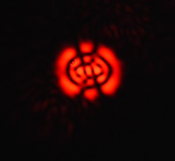
Created using a DMD
Laguerre-Gaussian modes
$\text{LG}_{p}^l(r, \phi, z) = \frac{1}{w(z)} \sqrt{\frac{2p!}{\pi (p + |l|)!}} \left(\frac{\sqrt{2} r}{\omega(z)}\right)^{|l|} L_p^{|l|}\left(\frac{2r^2}{\omega(z)^2}\right) \exp\left(-\frac{r^2}{\omega(z)^2}\right) \exp\left(-i \left(k z + k \frac{r^2}{2 R(z)} - l \phi - (2p + |l| + 1)\Psi(z)\right)\right)$
where r is the radius, $\omega_0$ represents the beam width at $z = 0$, $\omega(z) = \omega_0\sqrt{1 + z^2/z_R^2}$ describes the beam width, $R(z) = z + z^2_R/z$ is the radius of curvature of the phase front, $z_R = k\omega_0^2/2$ is the Rayleigh range and $\Psi = arctan(z/z_R)$ is the Gouy shift.
Code implementation
from optikit.Beam import Beam

Lag = Beam(type = 'LaguerreGauss',
            size = 5e-3,
            shape = 501,
            p = 2,
            l = 2,
            w0 = 1e-3,
            k = (2*np.pi/632.8e-9),
            z = 0)
Lag.plot_amplitude()
Hermite-Gaussian modes
$\text{HG}_{m}^n(x, y, z) = \frac{1}{w(z)} \sqrt{\frac{2}{\pi , 2^{n+m} , n! , m!}} , H_n\left(\frac{\sqrt{2} , x}{w(z)}\right) H_m\left(\frac{\sqrt{2} , y}{w(z)}\right) \exp\left(-\frac{x^2 + y^2}{w(z)^2}\right) \exp\left(-i \left(k z + (n + m + 1) \Psi(z) - \frac{k (x^2 + y^2)}{2 R(z)}\right)\right)$
where r is the radius, $\omega_0$ represents the beam width at $z = 0$, $\omega(z) = \omega_0\sqrt{1 + z^2/z_R^2}$ describes the beam width, $R(z) = z + z^2_R/z$ is the radius of curvature of the phase front, $z_R = k\omega_0^2/2$ is the Rayleigh range and $\Psi = arctan(z/z_R)$ is the Gouy shift.
Code implementation
from optikit.Beam import Beam

Herm = Beam(type = 'HermiteGaussian',
            size = 5e-3,
            shape = 501,
            n = 2,
            m = 2,
            w0 = 1e-3,
            k = (2*np.pi/632.8e-9),
            z = 0)
Herm.plot_amplitude()
Hologram generation
The slmpy module can be used to project the holograms in a SLM, the code implementation should be as bellow:
from optikit.Beam import Beam
import slmpy

Ince = Beam(type = 'InceGaussian',
            size = 5e-3,
            shape = 501,
            parity = 0,
            p = 2,
            m = 2,
            e = 2,
            w0 = 1e-3,
            k = (2*np.pi/632.8e-9),
            z = 0)

slm = slmpy.SLMdisplay()
Hologram = Ince.Beam.Hologam(gamma=np.pi/3000, theta = np.pi/4, save= True)
slm.updateArray(Hologram)
Propagator
The equation is solve numericaly by applying a transfer function.
$U(z) = \mathfrak{F}^{-1}\left\{H\cdot \mathfrak{F}\{U_0\}\right\}$
where $H = \exp\left(-i kz\sqrt{k_0^2 -\left(k_x^2+k_y^2\right)}\right)$ and $U_0$ represents the initial field.
Code implementation
The Propagator class supports as an input a np.ndarray ans OptiKit.Beam class
from optikit.optics import propagator
from optikit.Beam import Beam

Gauss = Beam(type = 'Gaussian',
            size = 2e-3,
            shape = 2**8,
            w0 = 1e-3,
            k = (2*np.pi/632.8e-9),
            z = 0)

Gauss.plot_amplitude()
Gauss_z = Propagator(beam= Gauss)
Gauss_z.propagate(zi = 1/2 * (2*np.pi/632.8e-9) * (1e-3 ** 2) , zn = 2**8)
Gauss_z.plot()
Stokes parameters
A classical way to measure the stokes paramters is the following:
| Polarizer axis angle | Wave plate fast axis angle | Power Measurement |
|---|---|---|
| $0°$ | - | $P_1$ |
| $90°$ | - | $P_2$ |
| $45°$ | - | $P_3$ |
| $45°$ | $0°$ | $P_4$ |
Stokes equations
- $S_0 = P_1 + P_2$
- $S_1 = P_1 - P_2$
- $S_2 = 2P_3 - S_0$
- $S_3 = S_0 - 2P_4$
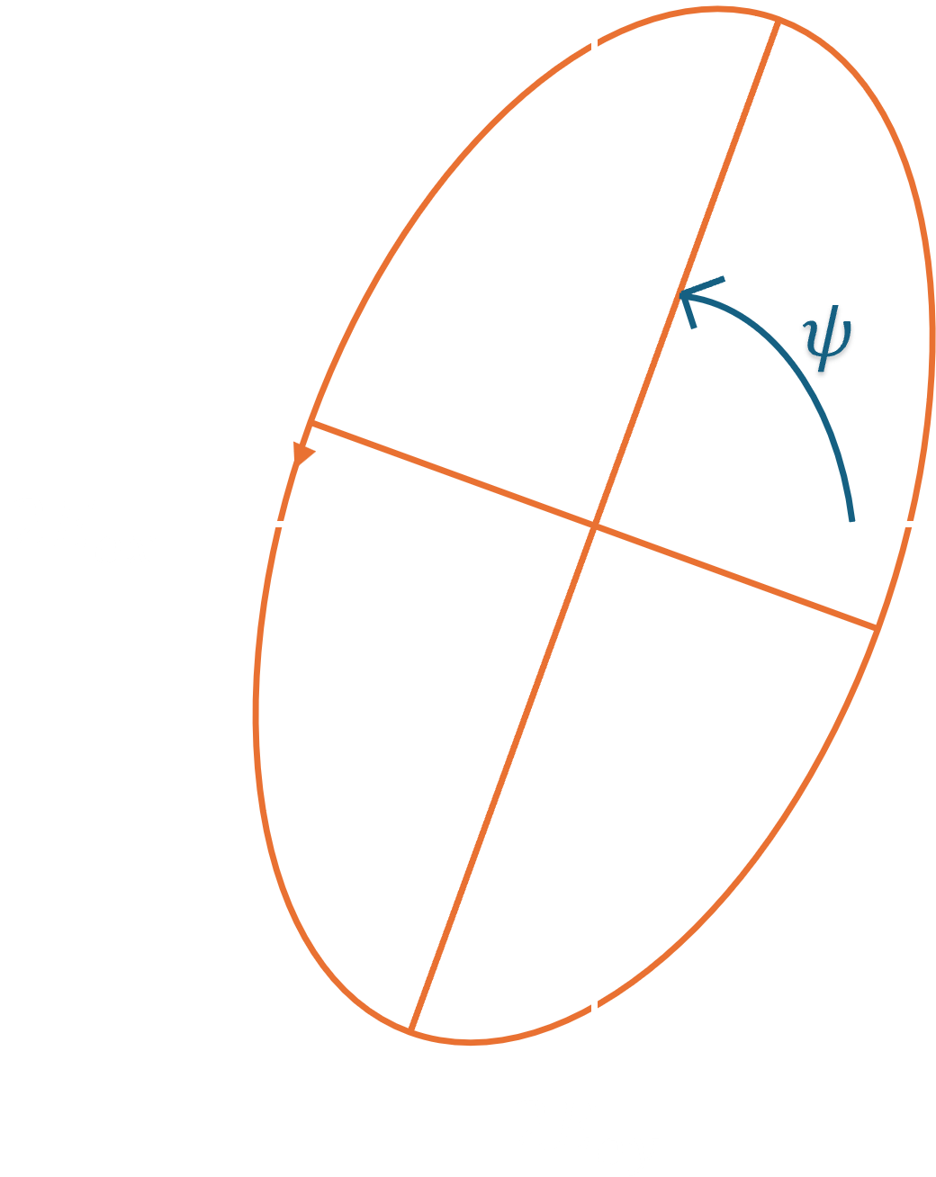
Ellipse Parameters
- $\psi = \frac{1}{2}\text{arctan}\left(\frac{S_2}{S_1}\right)$
- $E_{ox} = \sqrt{0.5(S_0 + S_1)}$
- $E_{oy} = \sqrt{0.5(S_0 - S_1)}$
Example
References
[1] R. W. Gerchberg and W. O. Saxton, “A practical algorithm for the determination of the phase from image and diffraction plane pictures”, Optik 35, 237 (1972).
[2] K. Mitchell, S. Turtaev, M. Padgett, T. Cizmár, and D. Phillips, “High-speed spatial control of the intensity, phase and polarisation of vector beams using a digital micro-mirror device”, Opt. Express 24, 29269-29282 (2016).
[3] Forbes A. 2014, Laser Beam Propagation: Generation and Propagation of Customized Light (London: Taylor and Francis).
[4] Bandres MA, Gutiérrez-Vega JC. Ince-Gaussian modes of the paraxial wave equation and stable resonators. J Opt Soc Am A Opt Image Sci Vis. 2004 May;21(5):873-80. doi: 10.1364/josaa.21.000873. PMID: 15139441.
[5] Beth Schaefer, Edward Collett, Robert Smyth, Daniel Barrett, and Beth Fraher "Measuring the Stokes polarization parameters," Am. J. Phys. 75, 163-168 (2007).
[6] Siegman, A. E. (1986). Lasers. Taiwan: University Science Books.
[7] Vallone, Giuseppe. (2015). On the properties of circular beams: normalization, Laguerre–Gauss expansion, and free-space divergence. Optics Letters. 40. 10.1364/OL.40.001717.
[8] Capps DM. Derivation and application of a Green function propagator suitable for nonparaxial propagation over a two-dimensional domain. J Opt Soc Am A Opt Image Sci Vis. 2019 Apr 1;36(4):563-577. doi: 10.1364/JOSAA.36.000563. PMID: 31044976.
To do
This project is still in development. New features will be added in upcoming versions.
1 maintainer

Metadata
1 maintainer
Release files for OptiKit 0.1.1a11
For a detailed explanation of source distributions (sdists) and built distributions (wheels), please see the package formats documentation.
Source distribution (sdist)
| File | Size | Uploaded | |
|---|---|---|---|
| optikit-0.1.1a11.tar.gz | 14.1 kB | Details |
Built distribution (wheel)
| File | Interpreter | ABI | Platform | Reset |
|---|---|---|---|---|
| OptiKit-0.1.1a11-py3-none-any.whl | Python 3 | none | any | Details |
Total release size: 33.6 kB
Release files / optikit-0.1.1a11.tar.gz
| Download URL | optikit-0.1.1a11.tar.gz |
|---|---|
| Size | 14.1 kB |
| Tags | Source |
|
SHA-256 checksum How to use checksums |
ff5f730311b91b0955cbb16d30dfcc3dddeee640ebaac3fd89c83957e5967713
|
|
BLAKE2b-256 checksum How to use checksums |
a66a0abf8d4891ec902270b29b8cd1de7c4e3aa4c68341d227bf54677379349d
|
| Upload date | |
|
Uploaded using Trusted Publishing? What is trusted publishing? |
No |
| Uploaded via |
twine/5.1.1 CPython/3.12.4
|
Release files / OptiKit-0.1.1a11-py3-none-any.whl
| Download URL | OptiKit-0.1.1a11-py3-none-any.whl |
|---|---|
| Size | 19.5 kB |
| Tags | Python 3 |
|
SHA-256 checksum How to use checksums |
a582158f5ace5b7440d1a640e914ab8448d4fa523a79740f642da9aebeee70fd
|
|
BLAKE2b-256 checksum How to use checksums |
96db6bbb7f79ed84f1d3881a1180debf2edfa3f72584247f88acef563fbc3285
|
| Upload date | |
|
Uploaded using Trusted Publishing? What is trusted publishing? |
No |
| Uploaded via |
twine/5.1.1 CPython/3.12.4
|














