Tools for piezoelectric transducer analysis.

Project description
PiezoLab
PiezoLab is a small Python package for working with piezoelectric impedance data and extracting Butterworth-Van Dyke ( BVD) equivalent circuit parameters from frequency sweeps.
It provides:
- An
Impedanceclass for turning magnitude/phase data into complex impedance and admittance - Automatic estimation of resonant and anti-resonant frequencies
- Initial BVD parameter extraction for
R1,C0,Qm,C1, andL1 - Optional nonlinear fitting with
scipy.optimize.curve_fit - A weighted least-squares fit for noisy or resonance-sensitive datasets
- Bundled sample datasets for quick testing and examples
Installation
PiezoLab can be installed with pip
pip install piezolab
For editable development installs, clone the repository and run:
pip install -e .
Quick Start
import matplotlib.pyplot as plt
from piezolab import Impedance, get_data
frequency, magnitude, phase_deg = get_data("clean_resonant_data")
impedance = Impedance(frequency, magnitude, phase_deg)
impedance.least_squares_fit(resonance_weight=100)
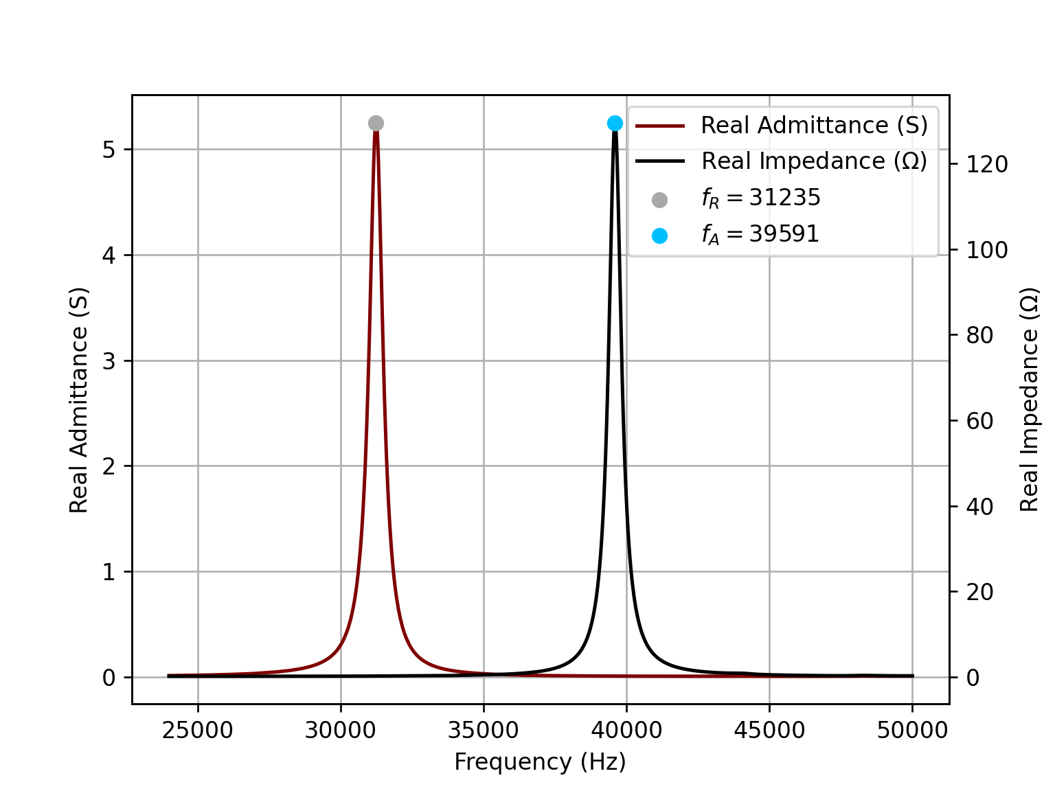
impedance.plot_real()
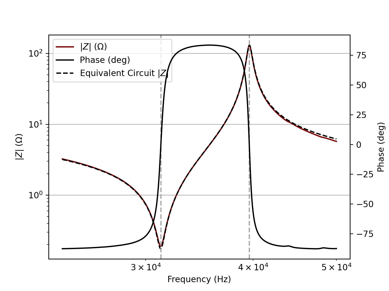
impedance.plot_impedance()
impedance.summarize()
plt.show()
This will show the real admittance and impedance plots as well as the fitted impedance magnitude and phase as shown below.
Data Model
Create an Impedance object from three NumPy arrays:
frequency: frequency in Hzimpedance_magnitude: impedance magnitude in ohmsimpedance_phase_deg: impedance phase in degrees
from piezolab import Impedance

imp = Impedance(frequency, impedance_magnitude, impedance_phase_deg)
During initialization, the class computes:
impedance_complexangular_frequencyadmittance_complexreal_impedancereal_admittanceadmittance_phase_deg
It also calls resolve_resonance() automatically to estimate the main BVD parameters.
Resolved Parameters
After initialization, these attributes are available:
resonant_frequency(fR)anti_resonant_frequency(fA)motional_resistance(R1)static_capacitance(C0)resonant_quality_factor(Qm)motional_capacitance(C1)motional_inductance(L1)
These values are first estimated directly from the measured impedance/admittance response, then can be refined with fitting.
Fitting Methods
curve_fit()
Uses scipy.optimize.curve_fit to fit the BVD model to the real and imaginary parts of the impedance.
imp.curve_fit()
Optional off-resonance capacitance constraint:
imp.curve_fit(off_res_cap=True)
imp.curve_fit(off_res_cap=120e-9)
Behavior:
off_res_cap=NoneorFalse: fitC0,C1,R1, andL1off_res_cap=True: estimate off-resonance capacitance from early low-frequency points and constrain the fitoff_res_cap=<float>: use a manually supplied off-resonance capacitance value
If your dataset does not provide enough off-resonance points with off_res_cap=True, then a warning will be issued as
the estimate may be inaccurate. In that case, consider manually providing the float value.
least_squares_fit()
Uses scipy.optimize.least_squares with nonnegative parameter bounds and optional weighting near resonance.
result = imp.least_squares_fit(
    resonance_weight=5.0,
    resonance_width=None,
    frequency_weights=None,
    off_res_cap=None,
)
Key options:
resonance_weight: increases the importance of points nearfRresonance_width: width of the resonance weighting window in rad/sfrequency_weights: custom weight array matching the frequency array shapeoff_res_cap: same constrained-fit options ascurve_fit()
This method is the better starting point when:
- the resonance region matters more than off-resonance behavior
- you want direct control over weighting
Plotting
plot_real()
Plots:
- real admittance vs frequency
- real impedance vs frequency
- markers for
fRandfA
fig, ax_admittance, ax_impedance = imp.plot_real()
plot_impedance()
Plots:
- measured impedance magnitude
- measured phase
- BVD equivalent circuit magnitude overlay
fig, ax_mag, ax_phase = imp.plot_impedance()
plot_impedance() overlays the model response generated from the current fitted or estimated parameters, so it is most
useful after curve_fit() or least_squares_fit().
Summary Output
summarize() prints the extracted BVD model parameters and an ASCII representation of the equivalent circuit:
imp.summarize()
The documented circuit is:
            |------|| C0 ------|
            |                  |
---o--------|                  |--------o---
            |                  |
            |---R1---L1---C1---|
Equivalent Circuit Evaluation
If you need the modeled impedance directly, use:
z_model = imp.equivalent_impedance(1j*imp.angular_frequency)
The argument is the complex frequency s, typically jω.
Bundled Sample Data
The package includes four sample datasets accessible through get_data():
clean_resonant_dataclean_sweep_datamessy_sweep_datamessy_resonant_data
Example:
from piezolab import get_data

frequency, magnitude, phase_deg = get_data("messy_sweep_data")
get_data() returns:
- frequency array
- impedance magnitude array
- impedance phase array in degrees
Example Scripts
The examples/ folder shows a few typical workflows:
examples/clean_data.py: clean resonant data with weighted least-squares fittingexamples/messy_data.py: messy sweep data with automatically estimated off-resonance capacitanceexamples/messy_resonant_data.py: messy resonant data with manually constrained off-resonance capacitance
Notes and Assumptions
- Input data should represent a single dominant resonance suitable for a BVD approximation.
- The automatic off-resonance capacitance estimate assumes the first low-frequency points are sufficiently far from resonance.
- If your low-frequency region is not truly off resonance, pass
off_res_capmanually instead of relying on automatic estimation. least_squares_fit()validates customfrequency_weightsshape and rejects invalid resonance weighting parameters.- Resonance detection is based on maxima in real admittance (
fR) and real impedance (fA).
Minimal Workflow
from piezolab import Impedance

imp = Impedance(frequency, magnitude, phase_deg)
imp.resolve_resonance()
imp.curve_fit()
imp.summarize()
Dependencies
PiezoLab depends on:
numpymatplotlibscipy
License
PiezoLab is licensed under the MIT License. See the LICENSE file for the full text.
Release history Release notifications | RSS feed

Download files
Download the file for your platform. If you're not sure which to choose, learn more about installing packages.
Source Distribution
Built Distribution
Filter files by name, interpreter, ABI, and platform.
If you're not sure about the file name format, learn more about wheel file names.
Copy a direct link to the current filters
File details
Details for the file piezolab-0.1.0.tar.gz.
File metadata
- Download URL: piezolab-0.1.0.tar.gz
- Upload date:
- Size: 106.3 kB
- Tags: Source
- Uploaded using Trusted Publishing? No
- Uploaded via: twine/6.2.0 CPython/3.12.0
File hashes
| Algorithm | Hash digest | |
|---|---|---|
| SHA256 |
76e650cb3d3c88f8e36e444db68fbdae32059ebe1824c12b6dac67394094be40
|
|
| MD5 |
464d2962f909cbf29212c1ed0e2fda38
|
|
| BLAKE2b-256 |
bcdaf43157958f9449a99360af786051e341b166b965bc180ea0b496bf07ecc0
|
File details
Details for the file piezolab-0.1.0-py3-none-any.whl.
File metadata
- Download URL: piezolab-0.1.0-py3-none-any.whl
- Upload date:
- Size: 102.3 kB
- Tags: Python 3
- Uploaded using Trusted Publishing? No
- Uploaded via: twine/6.2.0 CPython/3.12.0
File hashes
| Algorithm | Hash digest | |
|---|---|---|
| SHA256 |
34f5a40b85b855af7fdeb069f54834d4fec688f7702c0b951bac6fe765ec009f
|
|
| MD5 |
9c2a74530b962a317d55cd186be29f5a
|
|
| BLAKE2b-256 |
1fa2dd136476c00dc12e45fead80e22ffdf0e43fcb433b7829ade80a01d8bd1b
|


