
PolytopeGraphs in SageMath
This package allows to represent multi-dimensional continued fraction algorithms as polytopes graphs. It implements the Coulbois's and Fougeron's criterion to determine if there exists a unique ergodic invariant measure absolutely continuous with respect to Lebesgue.
Installation
You will need to install first Sagemath. For plots you also need to install the dot command from Graphviz. Then, you can install the polytope_graph package:
$ sage -pip install git+https://gitlab.com/davidsiukaev/polytopegraphs-in-sagemath.git
It can take a long time to compile since this package need first to install the badic package. It should be installed automatically with the previous command line.
Examples
Ergodic example
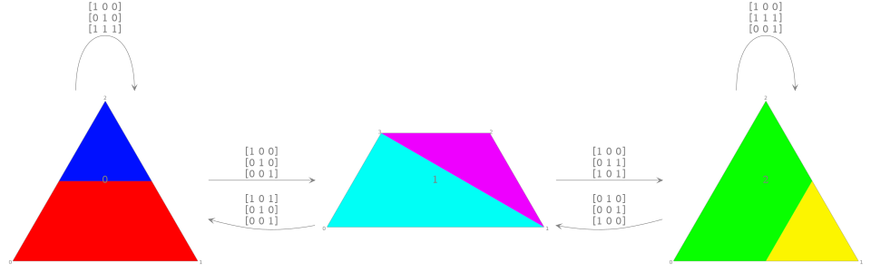
Define and plot a polytope graph:
sage: from polytope_graph import *
sage: m1 = matrix([[1,0,1],[0,1,1],[0,0,1]]).transpose()
sage: m2 = matrix([[1,0,0],[0,1,0],[0,0,1]]).transpose()
sage: m3 = matrix([[1,0,0],[0,1,0],[1,0,1]]).transpose()
sage: m4 = matrix([[1,0,1],[0,1,0],[0,1,1]]).transpose()
sage: m5 = matrix([[0,0,1],[1,0,0],[0,1,0]]).transpose()
sage: m6 = matrix([[1,1,0],[0,1,0],[0,1,1]]).transpose()
sage: s1_mat = matrix([[1,0,0],[0,1,0],[0,0,1]])
sage: s2_mat = matrix([[1,0,0,1],[0,1,1,0],[0,0,1,1]])
sage: b = PolytopeGraph([s1_mat, s2_mat, s1_mat], [(0,0,m1),(0,1,m2),(1,0,m3),(1,2,m4),(2,1,m5),(2,2,m6)])
sage: b.plot()
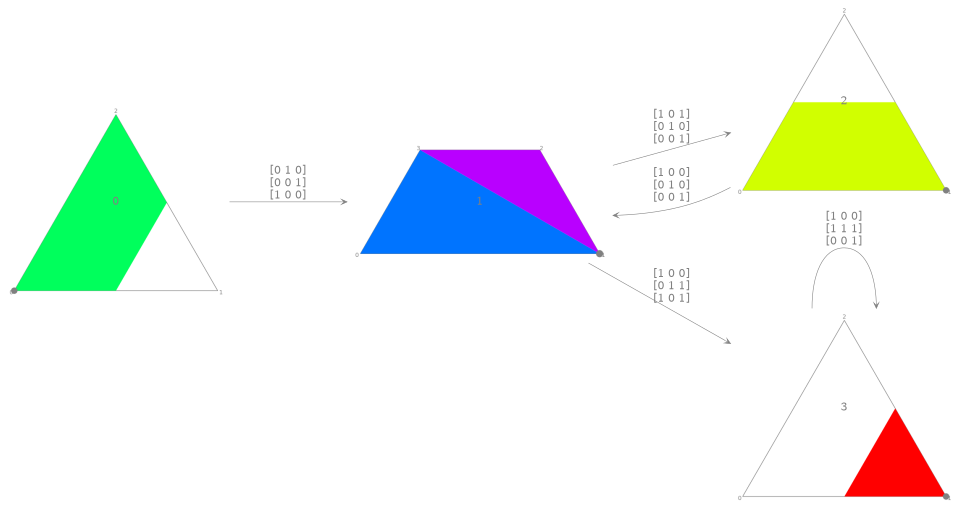
Compute a degenerate subgraph for a face with only one vertex:
sage: state = 2    # choose a state
sage: lf = b.faces(state)   # compute list of faces of the polytope of this state
sage: face = lf[4]           # choose one face
sage: b2 = b.degenerate_subgraph(state, face) # compute the degenerate subgraph for this face of this state
sage: b2.plot() # plot it
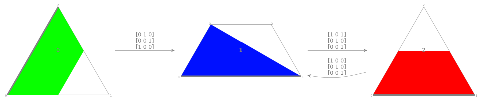
Compute another degenerate subgraph for a face of projective dimension 1:
sage: state = 2
sage: lf = b.faces(state)
sage: face = lf[2]
sage: b2 = b.degenerate_subgraph(state, face)
sage: b2.plot()
Check the Coulbois-Fougeron's criterion:
sage: b.Fougeron_Coulbois_criterion()
True
Non-ergodic example
sage: from polytope_graph import *
sage: m1 = matrix([[1,0,1],[0,1,0],[0,1,1]])
sage: m2 = matrix([[1,0,0],[0,1,1],[0,0,1]])
sage: m3 = matrix([[1,0,0],[0,1,0],[1,1,1]])
sage: m4 = matrix([[1,0,0],[0,1,0],[0,0,1]])
sage: s1 = matrix([[1,0,0,1],[0,1,1,0],[0,0,1,1]])
sage: s2 = matrix([[1,0,0],[0,1,0],[0,0,1]])
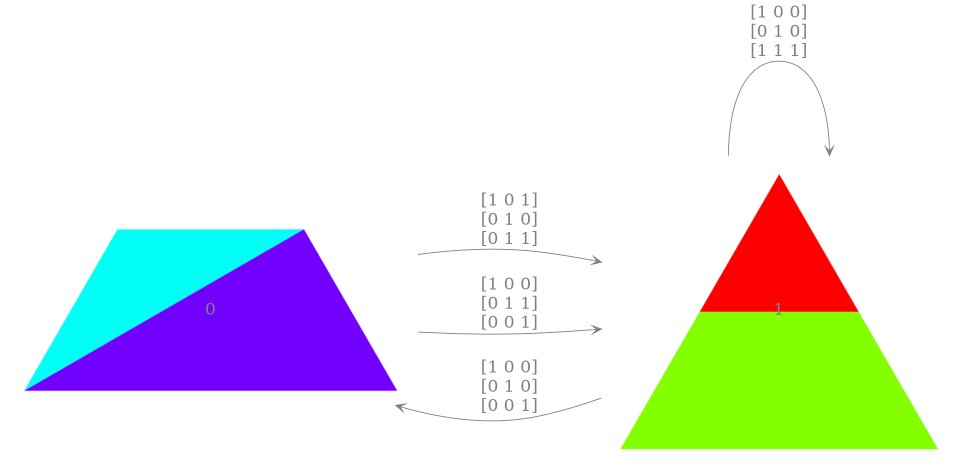
sage: a = PolytopeGraph([s1, s2], [(0,1,m1),(0,1,m2),(1,1,m3),(1,0,m4)])
sage: a.plot()
Check the Coulbois-Fougeron's criterion:
sage: a.Fougeron_Coulbois_criterion(verb = 1)
The criterion fails for the state 0 and the face:
[1]
[0]
[0]
False
sage: state = 0
sage: lf = a.faces(state)
sage: face = lf[6]
sage: face
[1]
[0]
[0]
sage: a2 = a.degenerate_subgraph(state, face)
sage: a2.plot()
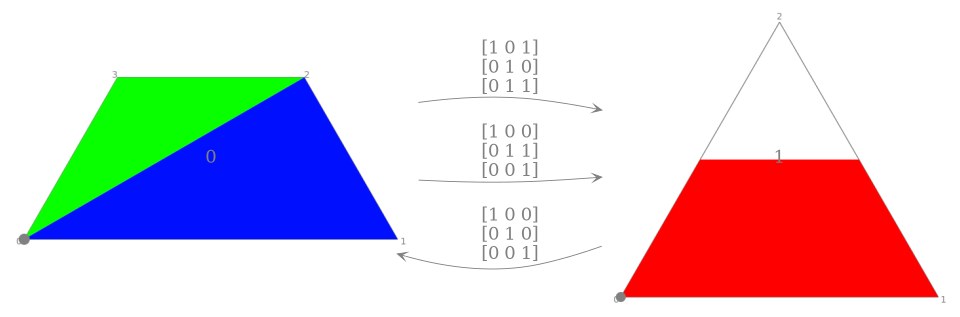
sage: a2.Fougeron_Coulbois_criterion_for_subgraph(verb=2)
[0, 1]
several outgoing edges from state 0
check inequality An inequality (0, -1, 1) x + 0 >= 0
check inequality An inequality (1, 0, 0) x + 0 >= 0
check inequality An inequality (0, 0, 1) x + 0 >= 0
check inequality An inequality (0, 1, -1) x + 0 >= 0
State 0 does not satisfies the criterion

False
Another ergodic example, with non non-negative matrices
sage: from polytope_graph import *
sage: s2 = matrix([[1,0,0],[0,1,0],[-1,1,1],[0,0,1]]).transpose()
sage: s1 = identity_matrix(3)
sage: m1 = matrix([[1,0,1],[0,1,1],[0,0,1]]).transpose()
sage: m2 = matrix([[1,0,0],[0,1,0],[1,0,1]]).transpose()
sage: m3 = matrix([[0,1,0],[-1,1,1],[0,0,1]]).transpose()
sage: a = PolytopeGraph([s1, s2], [(0,0,m1), (0,1,m2), (1,0,s1), (1,0,m3)])
sage: a.plot(colors='Set2')
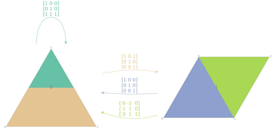
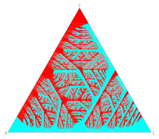
Iterations of the partition on each state:
sage: a.plot_state_partition2(1, 12)
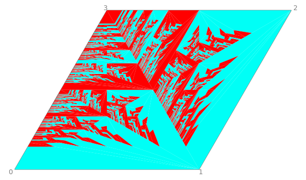
sage: a.plot_state_partition2(0, 12)
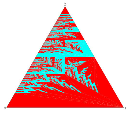
sage: s1 = identity_matrix(3)
sage: s2 = matrix([[1,0,0],[0,1,0],[0,1,1],[1,0,1]]).transpose()
sage: m1 = matrix([[0,0,1],[1,0,1],[0,1,1]]).transpose()
sage: m2 = matrix([[1,0,0],[1,1,0],[1,0,1]]).transpose()
sage: m3 = matrix([[1,1,0],[0,1,0],[0,1,1]]).transpose()
sage: m4 = matrix([[1,1,0],[0,1,1],[1,0,1]]).transpose()
sage: a = PolytopeGraph([s1, s2], [(0,0,m1), (0,1,s1), (1,0,m2), (1,0,m3), (1,0,m4)])
sage: a.plot_state_partition2(0, 13)
Change color, dark mode
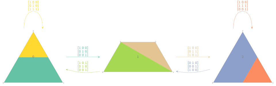
sage: from polytope_graph import *
sage: set_dark_mode(2) # transparent mode (set to 1 for dark mode, 0 for light mode)
sage: m1 = matrix([[1,0,1],[0,1,1],[0,0,1]]).transpose()
sage: m2 = matrix([[1,0,0],[0,1,0],[0,0,1]]).transpose()
sage: m3 = matrix([[1,0,0],[0,1,0],[1,0,1]]).transpose()
sage: m4 = matrix([[1,0,1],[0,1,0],[0,1,1]]).transpose()
sage: m5 = matrix([[0,0,1],[1,0,0],[0,1,0]]).transpose()
sage: m6 = matrix([[1,1,0],[0,1,0],[0,1,1]]).transpose()
sage: s1_mat = matrix([[1,0,0],[0,1,0],[0,0,1]])
sage: s2_mat = matrix([[1,0,0,1],[0,1,1,0],[0,0,1,1]])
sage: b = PolytopeGraph([s1_mat, s2_mat, s1_mat], [(0,0,m1),(0,1,m2),(1,0,m3),(1,2,m4),(2,1,m5),(2,2,m6)])
sage: b.plot(colors='Set2') # choose a color map
Convert win-lose or matrices graphs to PolytopeGraph
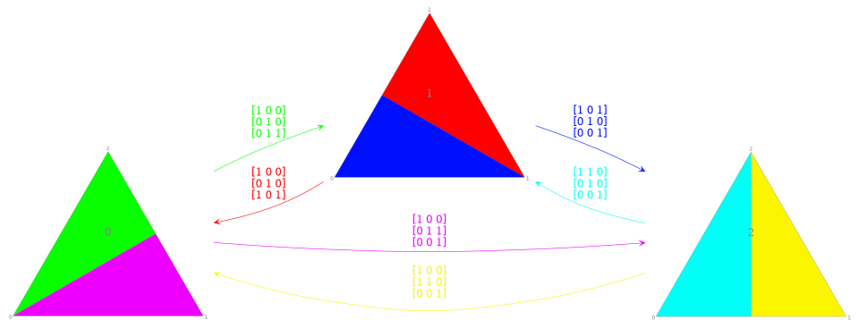
sage: from polytope_graph import *
sage: a = PolytopeGraph(dag.CassaigneWinLose())
sage: a.plot()
Compute the dual algorithm
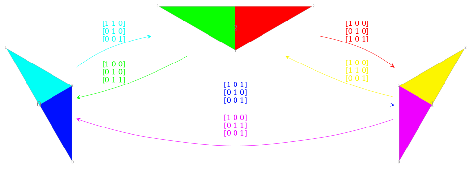
sage: ad = a.dual()
sage: ad.plot()
Convert a general algo to PolytopeGraph
sage: from polytope_graph import *
sage: a = dag.JacobiPerron()
sage: a = PolytopeGraph(a)
sage: a.plot()
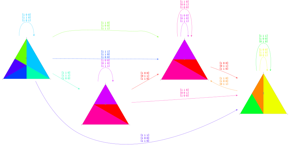
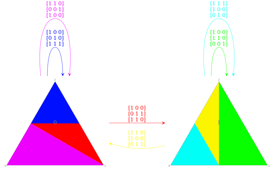
The graph is not strongly connected, so we need to restrict to a strongly connected component:
sage: c = a.strongly_connected_components()[0]    # choose the main strongly connected component
sage: a = a.subgraph(c)   # take the subgraph
sage: a.plot()
1 maintainer

Release files for polytope-graph 0.0.3
For a detailed explanation of source distributions (sdists) and built distributions (wheels), please see the package formats documentation.
Source distribution (sdist)
| File | Size | Uploaded | |
|---|---|---|---|
| polytope_graph-0.0.3.tar.gz | 22.4 kB | Details |
Release files / polytope_graph-0.0.3.tar.gz
| Download URL | polytope_graph-0.0.3.tar.gz |
|---|---|
| Size | 22.4 kB |
| Tags | Source |
|
SHA-256 checksum How to use checksums |
0b7311a5a7944619137f690c1b062b0f1cc23c43710641b933cff19f56d6682b
|
|
BLAKE2b-256 checksum How to use checksums |
d43bcd96ab19910e526b86852cf045d409d06788e6e113510b25d267350e4ab8
|
| Upload date | |
|
Uploaded using Trusted Publishing? What is trusted publishing? |
No |
| Uploaded via |
twine/6.2.0 CPython/3.12.12
|














