Radiative transfer and mass analysis for planetesimal formation simulations

Project description


protoRT
This is an open-source Python-based toolkit for 1D radiative transfer (with and without scattering) and mass analysis in numerical simulations of planetesimal formation. It computes the optical depth, outgoing intensity, and the mass excess due to optically thick regions in dust-rich environments. It supports mono and polydisperse models, with and without self-gravity. This code was used to research the mass budget problem in protoplanetary disks, see Godines et al. 2025.
Installation
The current stable version can be installed via pip:
$ pip install protoRT
Documentation
For technical details and examples of how to implement this program for numerical simulation analysis, check out our Documentation.
Getting Started
The code provides three main functionalities: Protoplanetary disk modeling, dust opacity calculations using DSHARP opacities (supports mono and polydisperse models), and the main class RadiativeTransferCube which conducts the radiative transfer, computing the optical depth, intensities, and resulting mass excess when optically thin emission is assumed.
To get started, a test dataset from a single-species streaming instability simulation without self-gravity, from Yang & Johansen (2014), taken at orbit 100, is provided and automatically loaded if no data is input. This is a shearing box with a cubic domain, set up with a Stokes number of 0.3 and a pressure gradient parameter of $\Pi$=0.05. The data will be loaded alongside the corresponding 1D coordinate axis array, in units of gas scale height (H).
from protoRT import rtcube

cube = rtcube.RadiativeTransferCube()

By default the class is instantiated with a gas column density (column_density) of $\Sigma_g$=10 (g/cm²), a temperature of T=30 (K), a gas scale height of H=5 (au), and a stokes number of stoke=0.3. The radiative transfer is also conducted at the 1 mm wavelength. There are a variety of simulation and model parameters to consider when using your own data, although note that a lot of these arguments are only required if analyzing multi-species simulations, with some others that are only necessary if the simulation is self-gravitating. Review the API documention for parameter details.
The configure class method will convert the simulation into physical units (cgs) and run through all the relevant calculations in order to perform the radiation transfer at the specified wavelength and compute the mass excess. When no opacities are input (kappa and/or sigma), the code will use the DSHARP opacities included in the compute_opacities module. When using the DSHARP opacities, ensure that the internal dust density of the dust grains (grain_rho) is the default value of 1.675 (g/cm³) to be consistent with the DSHARP dust model.
cube.configure()
Executing this method will automatically assign all of the relevant attributes including the optical depth at the output plane (tau), the corresponding intensity map (intensity), as well as the filling_factor, mass_excess, and the mass of each planetesimal in the simulation (proto_mass), if applicable. If analyzing multi-species models, a per-species density field will also be saved in the density_per_species class attribute; this is used to calculate particle-weighted opacities at each grid cell.
import numpy as np
import pylab as plt
fig, axes = plt.subplots(1, 2, figsize=(12, 5))
extent = [cube.axis[0], cube.axis[-1], cube.axis[0], cube.axis[-1]]
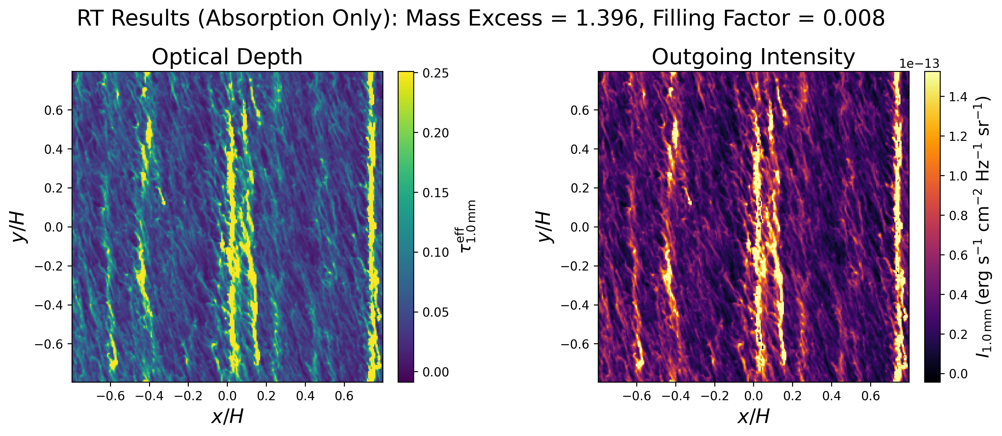
# Plot optical depth with robust scaling
med_tau = np.median(cube.tau)
std_tau = np.median(np.abs(cube.tau - med_tau))
vmin_tau, vmax_tau = med_tau - 3 * std_tau, med_tau + 10 * std_tau
im0 = axes[0].imshow(cube.tau, vmin=vmin_tau, vmax=vmax_tau, cmap='viridis', extent=extent, origin='lower', aspect='equal')
axes[0].set_title('Optical Depth', fontsize=18)
axes[0].set_xlabel(r'$x/H$', fontsize=16)
axes[0].set_ylabel(r'$y/H$', fontsize=16)
cbar0 = plt.colorbar(im0, ax=axes[0], fraction=0.046, pad=0.04)
cbar0.set_label(r'$\tau_{1.0\,\mathrm{mm}}^{\mathrm{eff}}$', fontsize=14)
# Plot intensity with robust scaling
med_int = np.median(cube.intensity)
std_int = np.median(np.abs(cube.intensity - med_int))
vmin_int, vmax_int = med_int - 3 * std_int, med_int + 10 * std_int
im1 = axes[1].imshow(cube.intensity, vmin=vmin_int, vmax=vmax_int, cmap='inferno', extent=extent, origin='lower', aspect='equal')
axes[1].set_title('Outgoing Intensity', fontsize=18)
axes[1].set_xlabel(r'$x/H$', fontsize=16)
axes[1].set_ylabel(r'$y/H$', fontsize=16)
cbar1 = plt.colorbar(im1, ax=axes[1], fraction=0.046, pad=0.04)
cbar1.set_label(r'$I_{1.0\,\mathrm{mm}} \, (\mathrm{erg}~\mathrm{s}^{-1}~\mathrm{cm}^{-2}~\mathrm{Hz}^{-1}~\mathrm{sr}^{-1})$', fontsize=14)
fig.suptitle(f'RT Results (Absorption Only): Mass Excess = {float(cube.mass_excess):.3f}, Filling Factor = {float(cube.filling_factor):.3f}', fontsize=18)
plt.tight_layout()
plt.show()
By default the scattering opacities are not considered in the radiative transfer, this is controlled via the include_scattering argument. The following shows the same analysis but with scattering.
IMPORTANT: The data cube is converted from code to physical units during the configuration, and is overwritten. As such, do not re-configure multiple times, instead re-instantiate the class object.
cube = rtcube.RadiativeTransferCube(include_scattering=True)
cube.configure()

# Plot
fig, axes = plt.subplots(1, 2, figsize=(12, 5))
extent = [cube.axis[0], cube.axis[-1], cube.axis[0], cube.axis[-1]]

# Plot optical depth with robust scaling
med_tau = np.median(cube.tau)
std_tau = np.median(np.abs(cube.tau - med_tau))
vmin_tau, vmax_tau = med_tau - 3 * std_tau, med_tau + 10 * std_tau
im0 = axes[0].imshow(cube.tau, vmin=vmin_tau, vmax=vmax_tau, cmap='viridis', extent=extent, origin='lower', aspect='equal')
axes[0].set_title('Optical Depth', fontsize=18)
axes[0].set_xlabel(r'$x/H$', fontsize=16)
axes[0].set_ylabel(r'$y/H$', fontsize=16)
cbar0 = plt.colorbar(im0, ax=axes[0], fraction=0.046, pad=0.04)
cbar0.set_label(r'$\tau_{1.0\,\mathrm{mm}}^{\mathrm{eff}}$', fontsize=14)

# Plot intensity with robust scaling
med_int = np.median(cube.intensity)
std_int = np.median(np.abs(cube.intensity - med_int))
vmin_int, vmax_int = med_int - 3 * std_int, med_int + 10 * std_int
im1 = axes[1].imshow(cube.intensity, vmin=vmin_int, vmax=vmax_int, cmap='inferno', extent=extent, origin='lower', aspect='equal')
axes[1].set_title('Outgoing Intensity', fontsize=18)
axes[1].set_xlabel(r'$x/H$', fontsize=16)
axes[1].set_ylabel(r'$y/H$', fontsize=16)
cbar1 = plt.colorbar(im1, ax=axes[1], fraction=0.046, pad=0.04)
cbar1.set_label(r'$I_{1.0\,\mathrm{mm}} \, (\mathrm{erg}~\mathrm{s}^{-1}~\mathrm{cm}^{-2}~\mathrm{Hz}^{-1}~\mathrm{sr}^{-1})$', fontsize=14)

fig.suptitle(f'RT Results (Absorption + Scattering): Mass Excess = {float(cube.mass_excess):.3f}, Filling Factor = {float(cube.filling_factor):.3f}', fontsize=18)
plt.tight_layout()
plt.show()
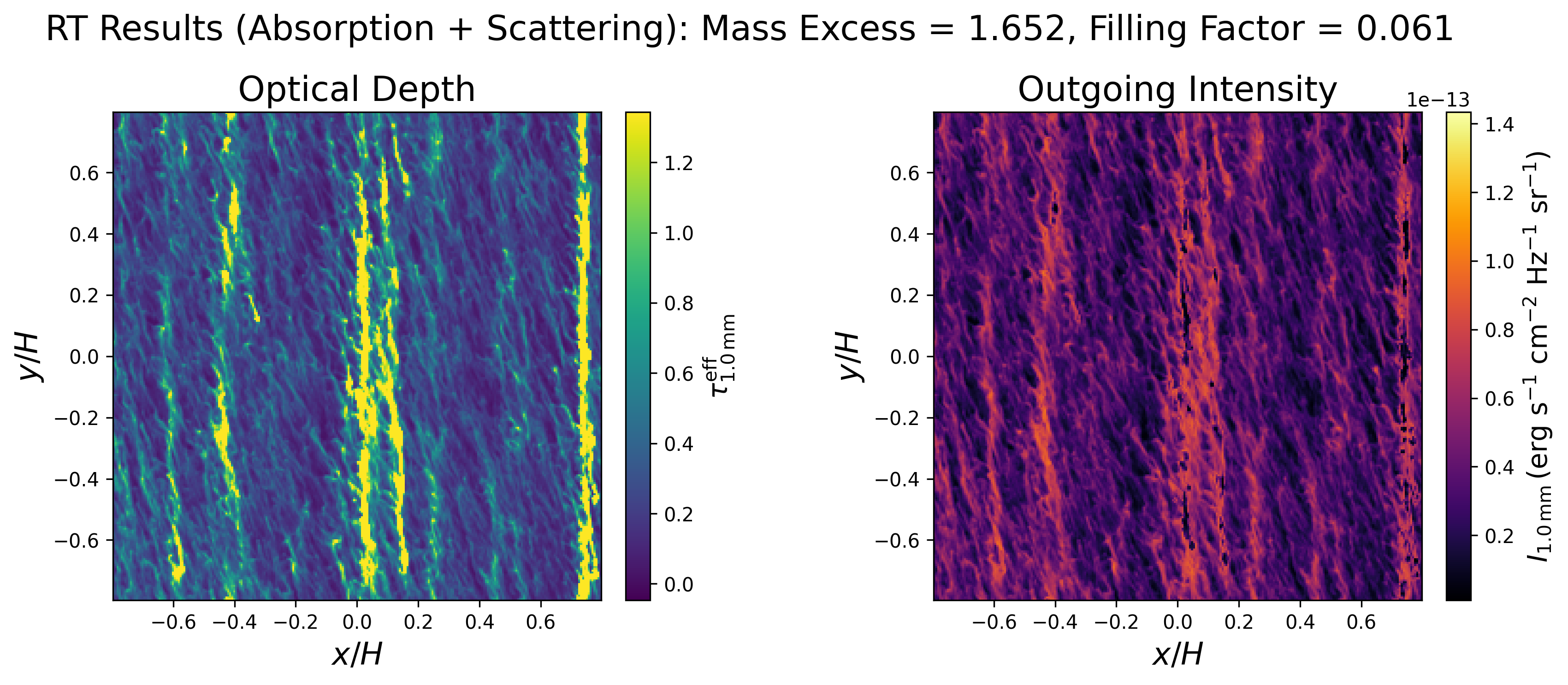
In this example we can see that scattering effects further suppress the emergent intensity and increase the mass excess and filling factor by approximately 16% and 13%, respectively.
To learn how to use the code, please review the following page which details how the program was used in Godines et al. 2025, which employed multi-species simulations with self-gravity, at three locations in the disk.
Citation
If you use this program in publication, we would appreciate citations to the paper, Godines et al. 2025.
How to Contribute?
Want to contribute? Bug detections? Comments? Suggestions? Please email us : godines@nmsu.edu, wlyra@nmsu.edu


Download files
Download the file for your platform. If you're not sure which to choose, learn more about installing packages.
Source Distribution
Built Distribution
Filter files by name, interpreter, ABI, and platform.
If you're not sure about the file name format, learn more about wheel file names.
Copy a direct link to the current filters
File details
Details for the file protort-1.0.2.tar.gz.
File metadata
- Download URL: protort-1.0.2.tar.gz
- Upload date:
- Size: 5.9 MB
- Tags: Source
- Uploaded using Trusted Publishing? No
- Uploaded via: twine/6.1.0 CPython/3.9.11
File hashes
| Algorithm | Hash digest | |
|---|---|---|
| SHA256 |
3f5a2c3938210860e4bd1f3ba9d139758e317f08f6a0fc7899c1b3fc6d2326b3
|
|
| MD5 |
9f2b2df1b586a6622d4f9d06be0e13f4
|
|
| BLAKE2b-256 |
9f765d34c98c36eae2db7d9a6c274e1fed8d4bae322da0f7e9f0beebc5e5e2b6
|
File details
Details for the file protort-1.0.2-py3-none-any.whl.
File metadata
- Download URL: protort-1.0.2-py3-none-any.whl
- Upload date:
- Size: 5.9 MB
- Tags: Python 3
- Uploaded using Trusted Publishing? No
- Uploaded via: twine/6.1.0 CPython/3.9.11
File hashes
| Algorithm | Hash digest | |
|---|---|---|
| SHA256 |
d00f1292b9949cd60cf17df7bb50a0a4f79649d35c6d452682b9bd26427e39b5
|
|
| MD5 |
dbebba69560e43b045b49ddf768da9a2
|
|
| BLAKE2b-256 |
43c9912131141965e19b4897b9ff49a817f9cf323f1b1add8024ebf7f723aac5
|


