
PyDRT
PyDRT is a lightweight Python implementation of the regularization-regression DRT with basis functions. The present code is published as part of the following work:
Leonhardt, et al. (2024). "Reconstructing the distribution of relaxation times with analytical basis functions" Journal of Power Sources 652, DOI: 10.1016/j.jpowsour.2025.237403
DRT can help you to deconvolute your impedance spectra, providing insights into the underlying processes of your electrochemical systems.
An example is illustrated below.
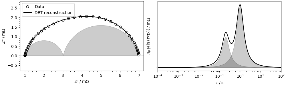
If this DRT implementation helps you with your research, please consider citing the reference above - this would be very helpful. :)
In case you want a more convenient DRT experience with a more user-friendly GUI, check out Polarographica (https://github.com/Polarographica/Polarographica_program), which was first to implement the Cole-Cole and Havriliak-Negami bases to the DRT algorithm.
To test the present code on synthetic impedance models, also check out https://github.com/robertleonhardt/PyImpedanceModel.
Usage
After instally PyDRT using
python -m pip install PyDRT
you can import it and us it as
import numpy as np
from pydrt import DebyeDRT

# Setup arbitrary model
frequency_model_Hz  = np.geomspace(1000, 0.001, 70)
impedance_model_Ohm = lambda omega: 1 + 2/(1 + (1j * 2 * np.pi * omega * 0.1) ** 0.99) + 4/(1 + (1j * 2 * np.pi * omega * 1) * 0.99)
impedance_model_Ohm = impedance_model_Ohm(frequency_model_Hz)

# Determine DRT
drt = DebyeDRT(frequency_model_Hz, impedance_model_Ohm, epsilon = 0.001)
The DRT primarily takes two inputs, a frequency vector and a complex-valued impedance vector of the same length.
The latter can be constructed in python by impedance_model_Ohm = real_part + 1j * imag_part.
Employing basis functions
The present DRT implementation approximates the DRT of a given measured (or synthetic) as a weighted sum (i.e., linear combination) of known basis functions. Four different types of bases are implemented in the given repository, usable as a class.
DebyeDRTis the basic DRT assuming ideal RC elementsGaussianDRTapproximates the processes to be normally distributed. The shape of the basis functions is defined by the full width at half maximum (FWHM), more details can be found here: https://en.wikipedia.org/wiki/Gaussian_functionColeColeDRTcan natively resemble depressed ZARC-elements (CPE in parallel to a resistor, more information: https://en.wikipedia.org/wiki/Cole-Cole_equation). The shape is defined by alpha.HavriliakNegamiDRTincorporates asymmetry into the ZARC element (see https://en.wikipedia.org/wiki/Havriliak-Negami_relaxation). In addition to alpha, a second parameter (beta) in implemented to account for the asymmetry.
More details on the used bases can be found in the reference at the top.
The code from the basic usage example can be adapted to employ other bases as:
import numpy as np
from pydrt import ColeColeDRT, DRTPeak

# Setup arbitrary model
frequency_model_Hz  = np.geomspace(1000, 0.001, 70)
impedance_model_Ohm = lambda omega: 1 + 2/(1 + (1j * 2 * np.pi * omega * 0.1) ** 0.9) + 4/(1 + (1j * 2 * np.pi * omega * 1) * 0.9)
impedance_model_Ohm = impedance_model_Ohm(frequency_model_Hz)

# Determine DRT
drt = ColeColeDRT(frequency_model_Hz, impedance_model_Ohm, alpha = 0.9)
The DRT object can the be used to further analyze the results. The following attributes might be useful:
# ...

# Vector containing the time constants
print(drt.tau_s)

# Vector containing the DRT and the DRT times the polarization resistance
print(drt.gamma)
print(drt.R_pol_Ohm * drt.gamma) # or in short, drt.gamma_hat_Ohm

# The reconstructed, complex DRT
print(drt.z_back_Ohm)
Furthermore, all bases (except the Debye basis) allow for convenient peak separation, which can be used as follows:
# ...

# Iterate through peaks
for peak in drt.get_separated_peak_list():
    print(peak.tau_s, peak.R_Ohm, peak.C_F)
The example scripts provided contain more details on the application of the DRT.
Determination of optimized shape and regularization parameters
The shape parameters of the non-Debye bases are typically defined by experience. This is also true for the Tikhonov regularization parameter (epsilon or lambda). It is, however, possible to optimize these parameters automatically.
For the regularization parameters, the code from the basic usage example is adapted accordingly to:
import numpy as np
from pydrt import DebyeDRT

# Setup arbitrary model
frequency_model_Hz  = np.geomspace(1000, 0.001, 70)
impedance_model_Ohm = lambda omega: 1 + 2/(1 + (1j * 2 * np.pi * omega * 0.1) ** 0.99) + 4/(1 + (1j * 2 * np.pi * omega * 1) * 0.99)
impedance_model_Ohm = impedance_model_Ohm(frequency_model_Hz)

# Determine DRT and optimize the regularization parameter
# Note that an object of the DebyeDRT class is passed to the static method "optimize_regularization_parameter"
drt = DebyeDRT.optimize_regularization_parameters(DebyeDRT(frequency_model_Hz, impedance_model_Ohm))
For shape parameters, the following code could be used:
import numpy as np
from pydrt import HavriliakNegamiDRT

# Setup arbitrary model
frequency_model_Hz  = np.geomspace(1000, 0.001, 70)
impedance_model_Ohm = lambda omega: 1 + 2/(1 + (1j * 2 * np.pi * omega * 0.1) ** 0.83) ** 0.6 + 4/(1 + (1j * 2 * np.pi * omega * 1) * 0.83) ** 0.6
impedance_model_Ohm = impedance_model_Ohm(frequency_model_Hz)

# Determine DRT and optimize the shape parameter
drt = HavriliakNegamiDRT.optimize_shape_parameters(HavriliakNegamiDRT(frequency_model_Hz, impedance_model_Ohm, tau_max_s = 1e1))
Since the Havriliak-Negami relaxation has two shape parameters (alpha and beta), the optimization takes some time (usually 30-45 seconds). For the other bases, this step is much faster.
Also note that regularization is typically not required when using dispersed bases (all classes except DebyeDRT).
But id is advised to consider validating this information for a specific use case.
Sources and acknowlegdements
Wan, T. H., et al. (2015). "Influence of the Discretization Methods on the Distribution of Relaxation Times Deconvolution: Implementing Radial Basis Functions with DRTtools." Electrochimica Acta 184: 483-499.
and, as the main source for the implementation of the Cole-Cole and Havriliak-Negami bases,
T. Tichter. https://github.com/Polarographica/Polarographica_program
1 maintainer

Metadata
1 maintainer
Release files for PyDRT 1.0
For a detailed explanation of source distributions (sdists) and built distributions (wheels), please see the package formats documentation.
Source distribution (sdist)
| File | Size | Uploaded | |
|---|---|---|---|
| pydrt-1.0.tar.gz | 14.8 kB | Details |
Built distribution (wheel)
| File | Interpreter | ABI | Platform | Reset |
|---|---|---|---|---|
| pydrt-1.0-py3-none-any.whl | Python 3 | none | any | Details |
Total release size: 33.5 kB
Release files / pydrt-1.0.tar.gz
| Download URL | pydrt-1.0.tar.gz |
|---|---|
| Size | 14.8 kB |
| Tags | Source |
|
SHA-256 checksum How to use checksums |
50b8f54b651195687a80d34eccd15d7c7a47d9813c7a226a2f6f069a208fc55e
|
|
BLAKE2b-256 checksum How to use checksums |
4b60ff30e3287f29283e41827bab0fa959b7ba0304592304471fe0c339acbaa3
|
| Upload date | |
|
Uploaded using Trusted Publishing? What is trusted publishing? |
No |
| Uploaded via |
twine/6.1.0 CPython/3.12.11
|
Release files / pydrt-1.0-py3-none-any.whl
| Download URL | pydrt-1.0-py3-none-any.whl |
|---|---|
| Size | 18.7 kB |
| Tags | Python 3 |
|
SHA-256 checksum How to use checksums |
2687d69afbd7e4c4bf55cfea5315d8e2cf3608565a5da80ee9432538ae5d88fb
|
|
BLAKE2b-256 checksum How to use checksums |
458ea985098046987fe01e5f2ff91a5e6208cf846de5ee30663df216002ab5c9
|
| Upload date | |
|
Uploaded using Trusted Publishing? What is trusted publishing? |
No |
| Uploaded via |
twine/6.1.0 CPython/3.12.11
|













