
PythonAQ



Air quality data analysis and visualisation for Python, following the R openair package. Download data from the UK monitoring networks and NOAA, average and condition it properly, and produce interactive Plotly figures.
Every figure in this manual is generated by
examples/build_readme_figures.py from real
AURN data for Leeds Centre, 2022–2025 — so what you see is what the package
actually renders.
Contents
- Installation
- Quick start
- Conditioning with
type - Getting data
- Directional analysis — how concentrations relate to wind
- Time series and trends
- Distributions and relationships
- Model evaluation
- Data utilities
- Meteorological helpers
- Relationship to openair
- Guide
- Worked example
- Development
- Releasing
- Licence
Installation
git clone https://github.com/chris-r-uol/PythonAQ.git
cd PythonAQ
pip install -e .
The package is then importable from anywhere:
from PythonAQ import import_aq_meta, wind_rose
Optional extras
Some features carry dependencies deliberately kept out of the core install:
pip install -e '.[calendar]'  # the calendar plot
pip install -e '.[app]'       # the Streamlit demo application
pip install -e '.[dev]'       # test and lint tooling
pip install -e '.[docs]'      # static image export, for rebuilding this manual
A caveat on the
calendarextra. It needsplotly-calplot, which pinsnumpy<2andplotly<6and does not work on pandas 3. Installing it will constrain the rest of your environment, which is whycalendaris the only function unavailable from a plainpip install -e .— and why it raises a helpfulImportErrorrather than failing at import time.
Dependencies
Python 3.9+, with numpy, pandas, scipy, plotly, requests, rdata, scikit-learn, statsmodels, pymannkendall and pygam.
Quick start
from PythonAQ import download_aurn_data, polar_plot, time_variation

# Four years of hourly data for Leeds Centre
df = download_aurn_data('LEED', 2022, 2025, 'aurn')

polar_plot(df, conc_col='NO2').show()
fig, summary = time_variation(df, 'NO2')
fig.show()
Most plotting functions return a Plotly Figure. Several also return a
DataFrame of the values behind the plot, so you can check or reuse the
numbers rather than reading them off a chart.
Conditioning with type
Nearly every plotting function takes type, which splits the data and draws
one panel per level. openair introduces this in chapter 2, before any plotting
chapter, because it applies to all of them.
polar_plot(df, conc_col='NO2', type='season')
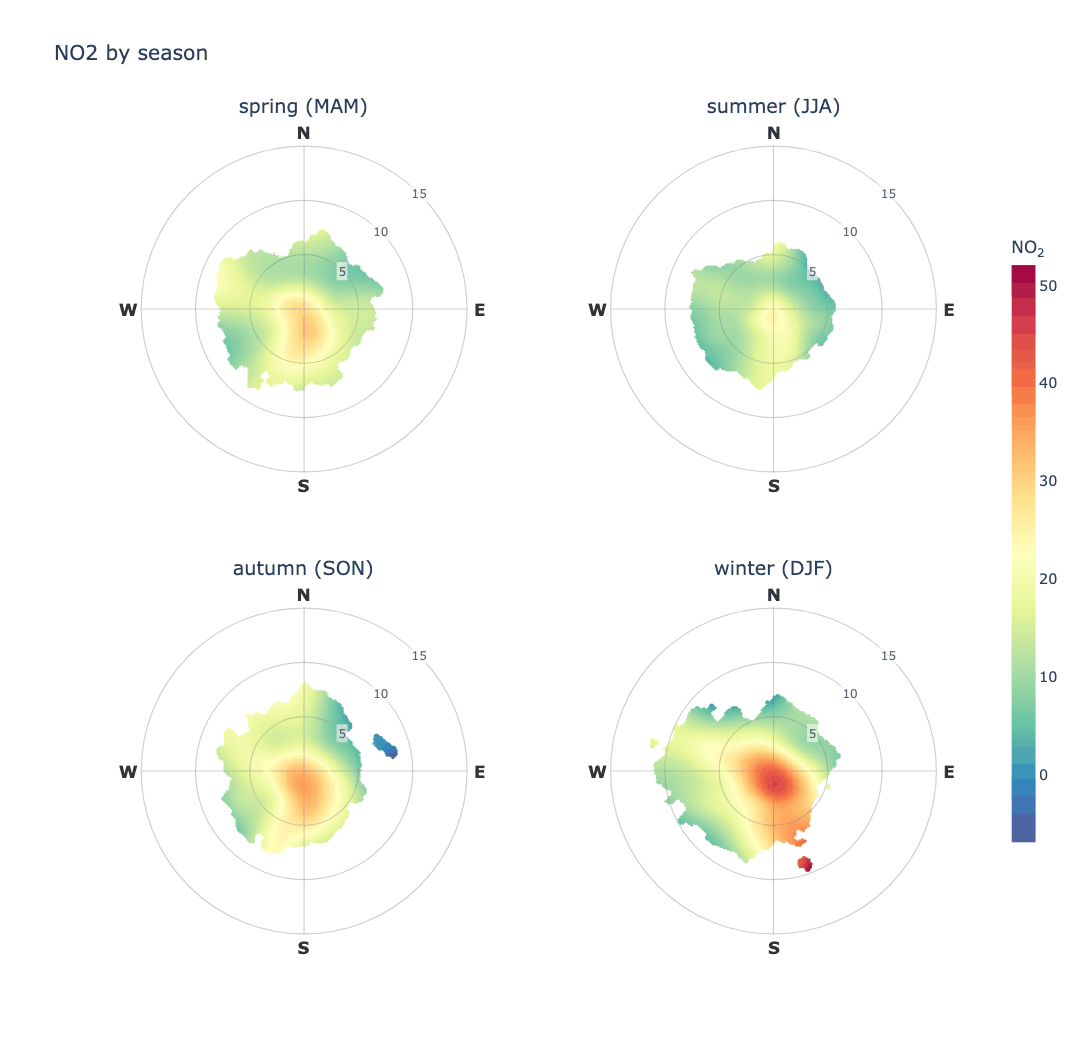
NO₂ at Leeds Centre is worst in winter and cleanest in summer, and the southerly arm is present year-round but strongest in the colder months.
type accepts anything cut_data understands:
type |
Panels |
|---|---|
'year', 'month', 'season' |
one per year, month or season |
'weekday', 'weekend' |
one per day, or weekday against weekend |
'hour', 'daylight' |
one per hour, or daylight against night |
'wd' |
one per compass sector |
| any numeric column | one per quantile, n_levels of them |
Alongside it: ncols for panels per row, hemisphere for season definitions,
n_levels for quantile counts, and panel_height.
Panels share one colour scale and one set of axis limits, so they can actually be compared — otherwise the same colour, or the same radius, would mean different things in different panels. Any other argument is passed to every panel, so a data-driven limit can be fixed across them explicitly:
# Without ws_limit each season sets its own radial extent from its own
# 99th percentile, and the rings stop being comparable.
polar_plot(df, conc_col='NO2', type='season', ws_limit=12)
Conditioning never changes what a function returns: polar_plot gives a
figure with or without type, and wind_rose gives a (figure, DataFrame)
pair either way, with the summary gaining a column naming the level.
Getting data
import_aq_meta
Site metadata for a UK monitoring network.
from PythonAQ import import_aq_meta

metadata = import_aq_meta('aurn')
source(str):'aurn','saqn','aqe','waqn'or'ni'.
Returns a DataFrame with site_id, site_name, location_type, latitude,
longitude, zone, local_authority and operating dates.
download_aurn_data
Hourly observations for one site across a range of years.
from PythonAQ import download_aurn_data

df = download_aurn_data(site='LEED', start_year=2022, end_year=2025, source='aurn')
site(str),start_year(int),end_year(int),source(str).
Returns a combined DataFrame, one row per hour, with a date_time column and
whichever pollutants the site measures.
download_noaa_data and parse_noaa_data
Meteorology from NOAA's Integrated Surface Database.
from PythonAQ import download_noaa_data

met = download_noaa_data(station_code='033440-99999', year_start=2022, year_end=2025)
parse_noaa_data does the decoding and is called for you by
download_noaa_data; call it directly if you have raw ISD CSVs. It splits the
packed comma-separated fields, clears the documented missing-value sentinels
before applying the ×10 scaling, resamples to hourly means, and derives
relative humidity.
Returns air_temp (°C), ws (m/s), wd (degrees), dew_point (°C),
atmospheric_pressure (hPa) and relative_humidity (%).
map_sites
Locate monitoring sites.
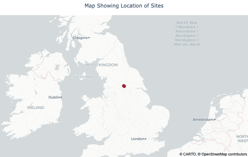
from PythonAQ import map_sites

map_sites(metadata, sites=['LEED', 'LED6']).show()
map_style(str): base tiles.'carto-positron'(default) and'carto-darkmatter'are muted OpenStreetMap-derived styles, light and dark, which keep the markers legible;'open-street-map'is the full-colour standard style, which competes with the data. None need an access token.zoom(int),marker_colour(str).
Directional analysis
How concentrations vary with wind speed and direction — the most direct way to ask where pollution is coming from.
polar_plot
Concentration as a function of both wind speed (radius) and direction, smoothed with a tensor-product GAM.
from PythonAQ import polar_plot

polar_plot(df, conc_col='NO2').show()
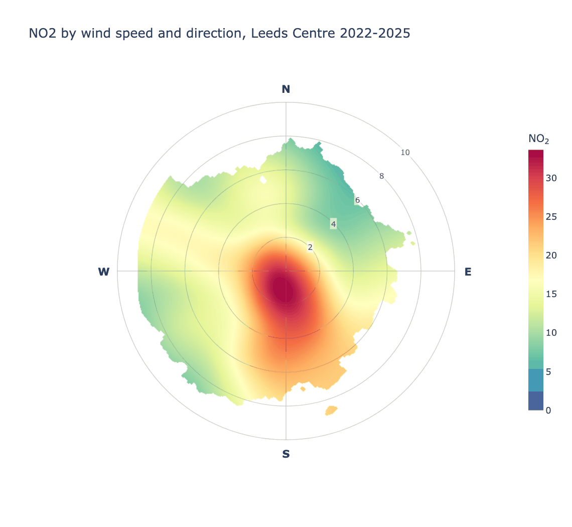
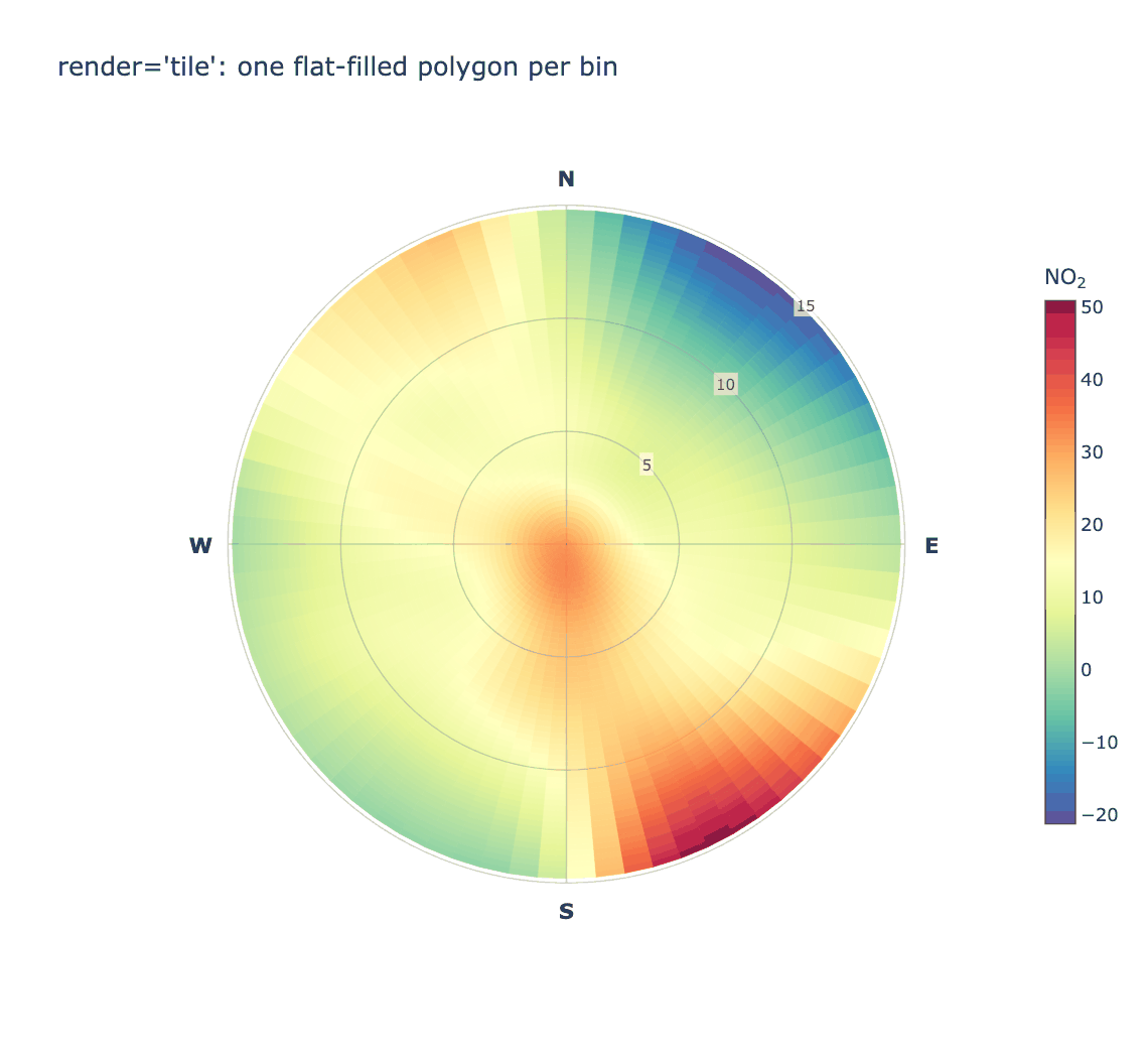
Reading this one: NO₂ at Leeds Centre — an urban background site — peaks at the centre of the plot, at low wind speeds, the signature of nearby ground-level sources accumulating under calm conditions rather than of a single distant stack. Concentrations stay elevated towards the south and south-west, and fall away to the north-east at higher wind speeds where cleaner air dilutes them.
Parameters
conc_col(str): concentration column.render(str):'raster'(default) draws one continuous surface,'contour'filled bands,'tile'the original one-polygon-per-bin rendering.resolution(int): grid points per axis, default 300. Higher is smoother and slower.ws_limit(str or float): radial extent.'auto'(default) uses the 99th percentile of wind speed,'max'the full observed range, or give a number.min_count(int): minimum observations per bin, and the local density required for a grid cell to be drawn.exclude_missing(bool),exclude_distance(float): blank grid areas too far from any observation, rather than extrapolating into empty sectors.uncertainty(float): confidence width, e.g.0.95, for blanking regions where the prediction interval exceeds the prediction.upper_limit(float): blank predictions above this concentration.
On rendering. The surface is predicted onto a regular Cartesian grid in
wind-component space and drawn as a single interpolated raster, which is what
openair does via lattice's levelplot.
polar_plot(df, conc_col='NO2', render='contour').show()
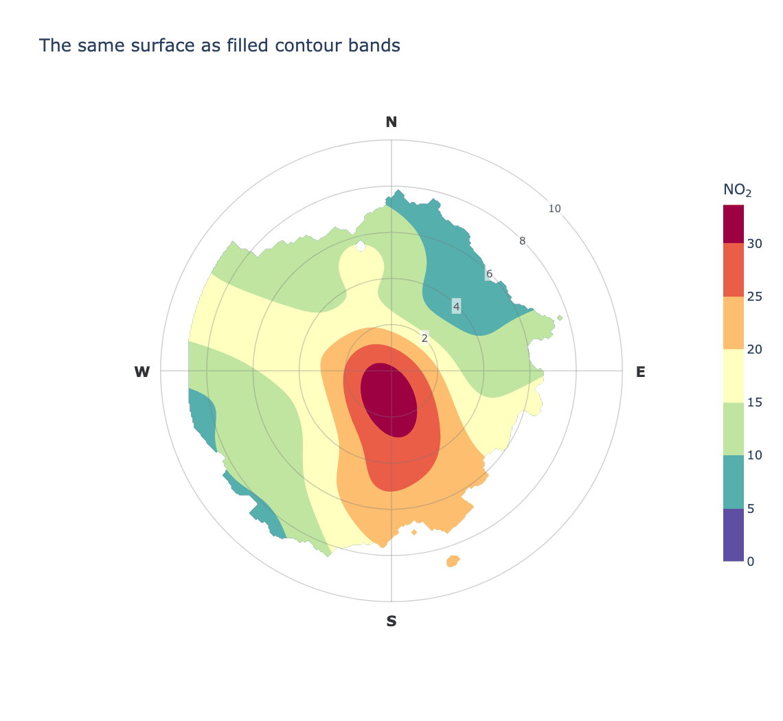
The old behaviour is still available, and shows why the default changed — drawing one flat-filled polygon per bin looks blocky however smooth the underlying fit is, because nothing interpolates between neighbouring cells:
polar_plot(df, conc_col='NO2', render='tile').show()
wind_rose
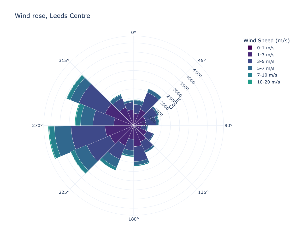
Wind speed and direction distribution.
from PythonAQ import wind_rose

fig, summary = wind_rose(df, group_by='none')
group_by(str):'none','year'or'quartile'.quartile_col(str): column to split on whengroup_by='quartile'.mode(str):'count'or'percentage'.direction_bins(int),speed_bins(list): binning.
Returns the figure and a summary DataFrame.
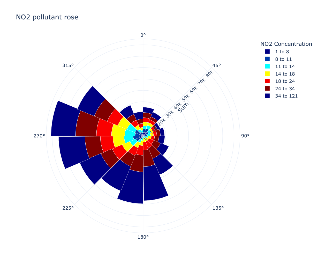
pollutant_rose
Concentration by wind direction, banded by concentration.
from PythonAQ import pollutant_rose

fig, summary = pollutant_rose(df, pollutant='NO2')
percentile_rose
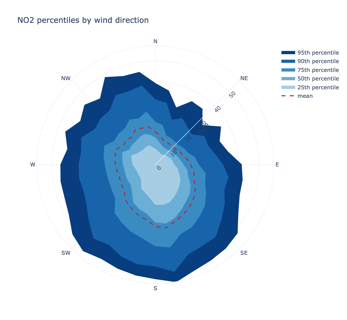
How the distribution, not just the mean, varies with direction. Useful when a source only shows up in the tail.
from PythonAQ import percentile_rose

fig, summary = percentile_rose(df, 'NO2', percentile=[25, 50, 75, 90, 95])
percentile(sequence): percentiles to draw.direction_bins(int): wind direction sectors, default 36.fill(bool),mean_line(bool): styling.statistic(str):'percentile'(default) or'cpf', below.cpf_threshold(float): concentration defining "high" for the CPF; defaults to the givenpercentileof the observations.
The conditional probability function
statistic='cpf' gives, for each wind sector, the proportion of observations
above a threshold:
percentile_rose(df, 'NO2', statistic='cpf', percentile=95)
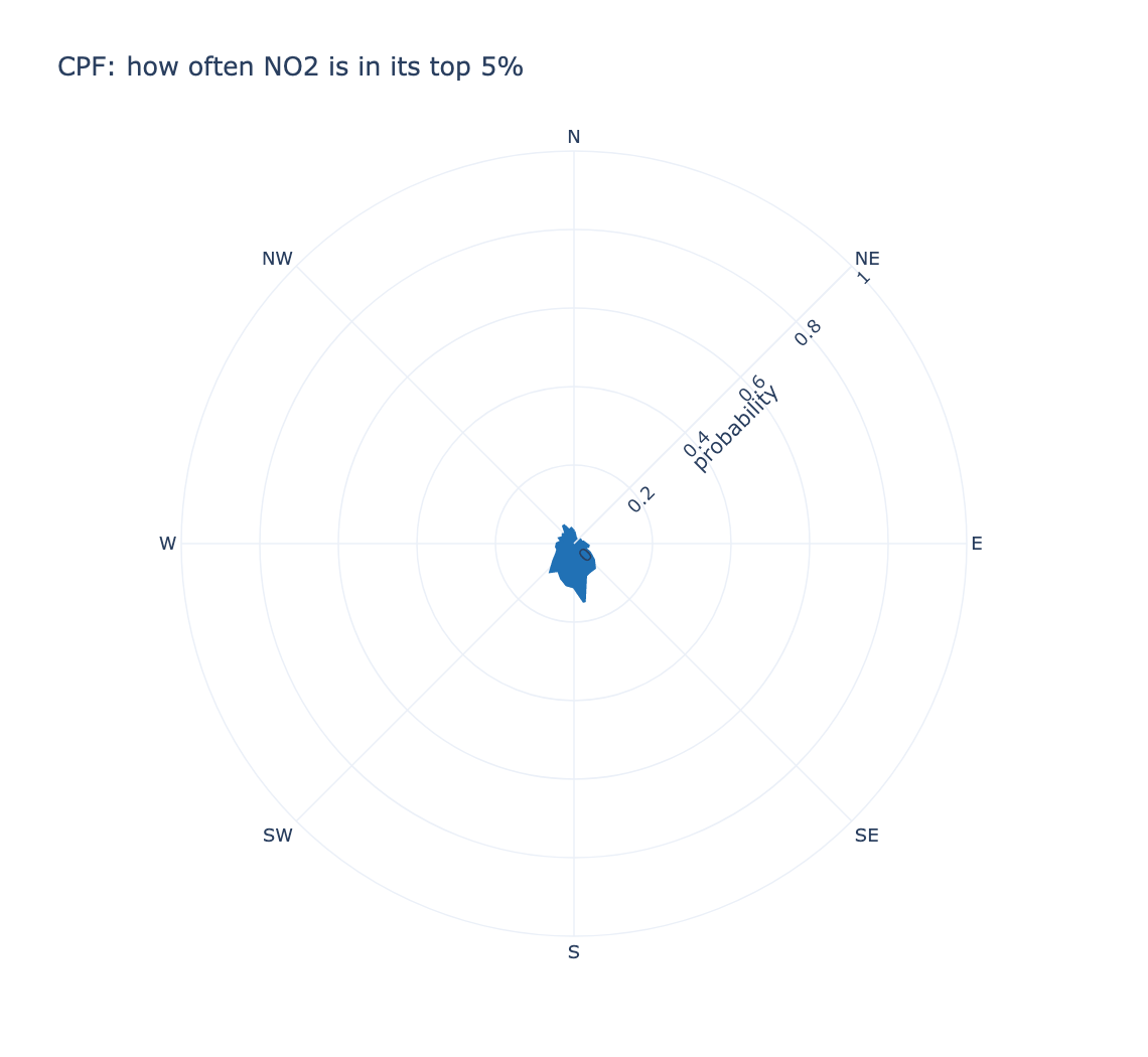
This asks when the wind comes from here, how often is the concentration high? — a different question from the directional mean, and one that finds sources a mean misses when they are intermittent. A sector that is usually clean but occasionally very dirty has an unremarkable mean and a high CPF.
The threshold is taken over the whole record rather than per sector, so every sector is judged against one definition of "high", and the radial axis is fixed to 0–1 so two sites can be compared by eye.
polar_frequency_plot
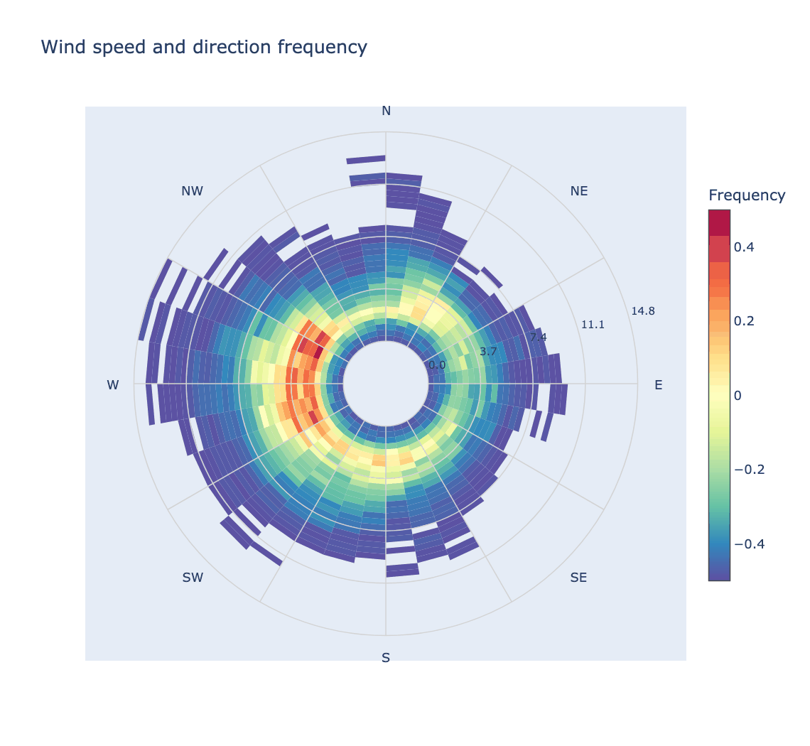
How often each wind speed and direction combination occurs — worth checking
alongside polar_plot, since a striking feature in a sector with almost no data
is not a finding.
from PythonAQ import polar_frequency_plot

polar_frequency_plot(df, separate_by_year=False).show()
polar_annulus
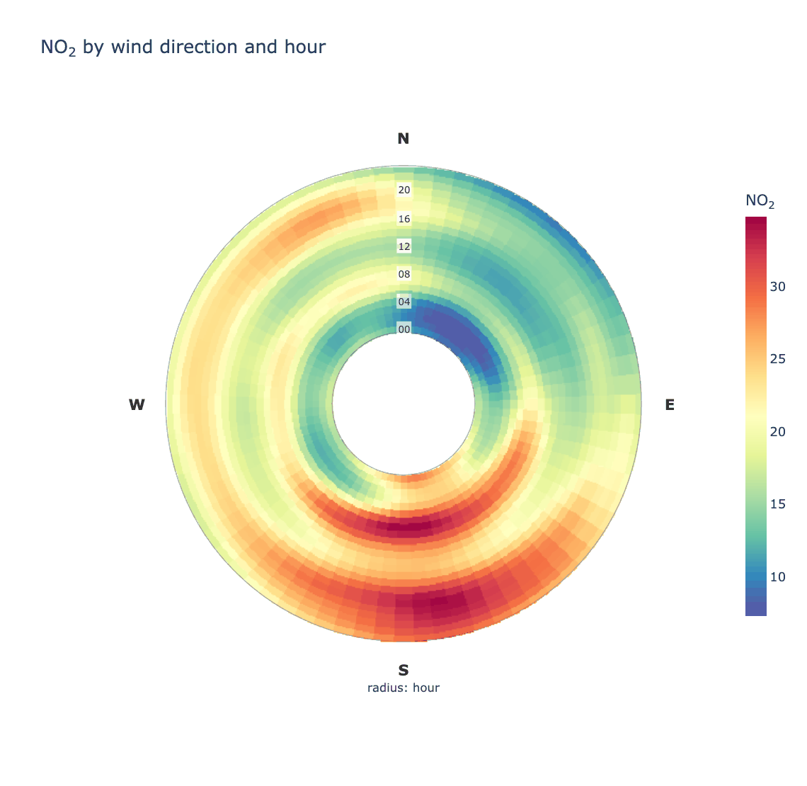
Wind direction around the ring, a temporal variable through it. For sources that only appear at certain hours or in certain months, which a plain polar plot averages away.
from PythonAQ import polar_annulus

fig, summary = polar_annulus(df, 'NO2', period='hour')
period(str): radial variable —'hour'(default),'month','weekday','season'or'trend'(one ring per year).inner_radius(float): size of the hole, so the innermost ring is not squeezed to nothing.smooth(bool),sigma(tuple): smoothing, which wraps at the cyclic edges so there is no seam at north.
polar_cluster
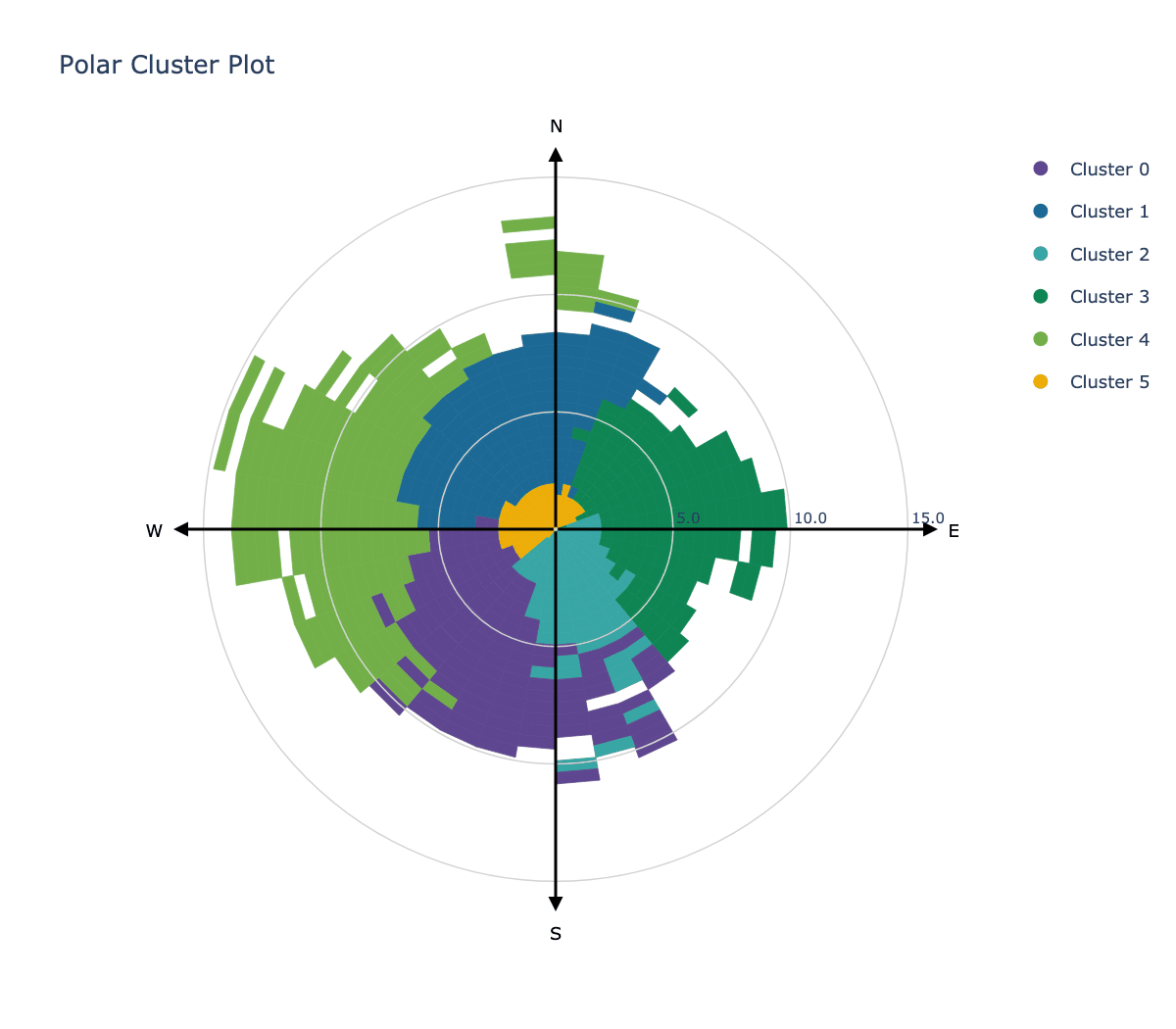
K-means clustering in polar coordinates, to group conditions that behave alike.
from PythonAQ import polar_cluster

polar_cluster(df, feature_cols=['NO2', 'PM10', 'O3'], n_clusters=6).show()
Time series and trends
time_variation
The four-panel temporal summary: hour of day split by weekday, day of week, hour of day, and month of year, each with bootstrap confidence intervals.
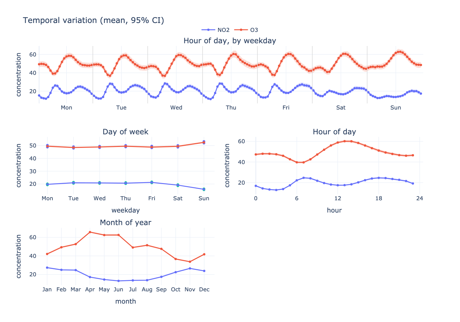
from PythonAQ import time_variation

fig, summary = time_variation(df, ['NO2', 'O3'], random_state=42)
At Leeds Centre NO₂ peaks at 07:00, runs about 3 µg/m³ lower at weekends, and is roughly twice as high in winter as in summer. O₃ moves the opposite way on all three axes, which is the expected titration relationship.
Parameters
pollutant(str or list): one or more columns.statistic(str):'mean'or'median'.conf_int(float): confidence level, default0.95.n_boot(int): bootstrap replicates (openair'sB), default 100.normalise(bool): divide each series by its mean, to compare shapes across variables on different scales.ci(bool): draw the confidence bands.random_state(int): seed, for reproducible intervals.
Returns the figure and a long-format DataFrame of every plotted statistic.
theil_sen_plot
Non-parametric trend estimate with confidence intervals and a Mann-Kendall significance test.
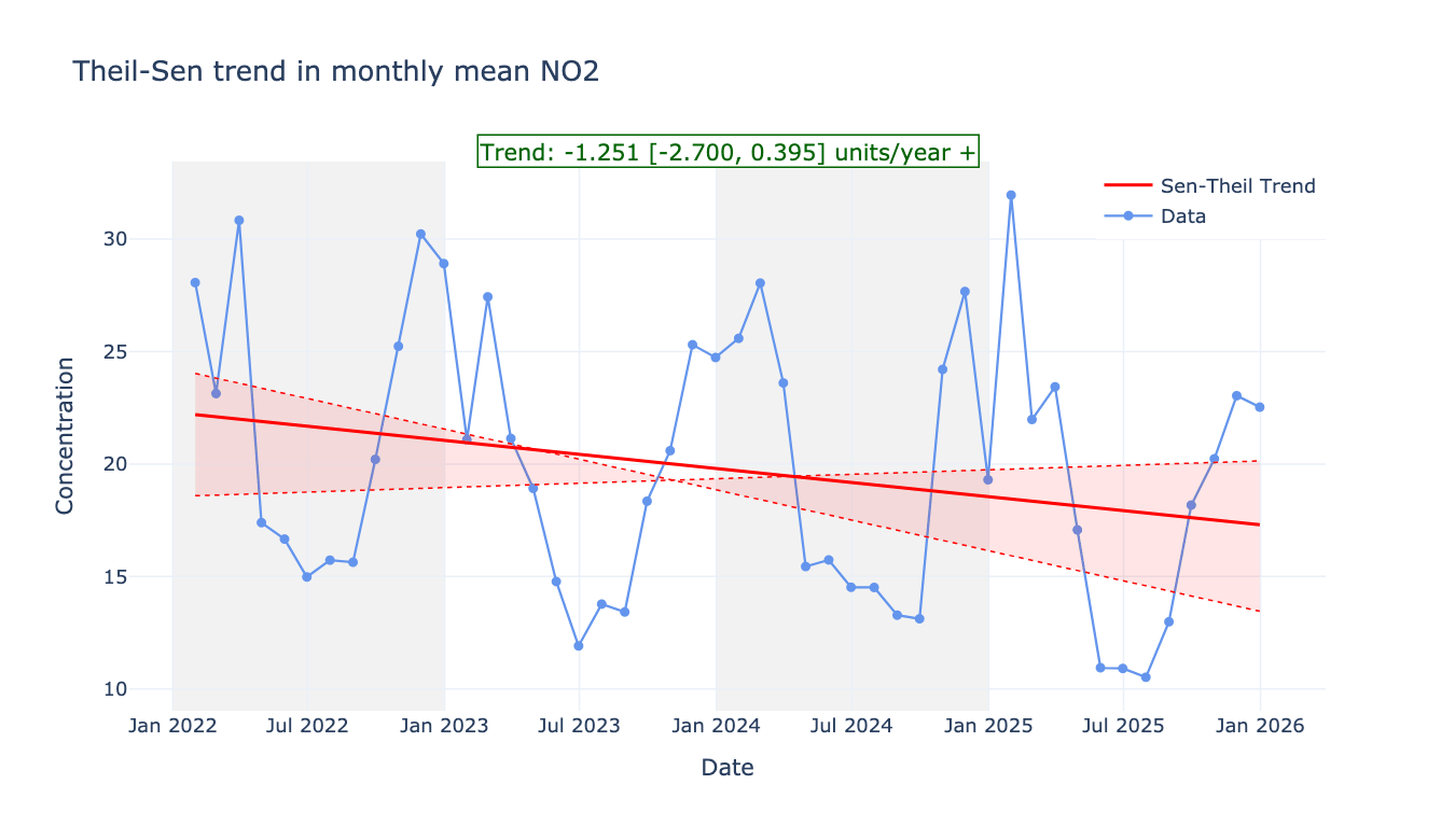
from PythonAQ import theil_sen_plot

theil_sen_plot(df, pollutant_col='NO2', agg_freq='ME').show()
agg_freq(str): averaging period before fitting, e.g.'ME'.deseason(bool): remove the seasonal cycle via STL first.alpha(float): significance level.
smooth_trend_plot
A GAM smooth rather than a straight line, for trends that are not monotonic.
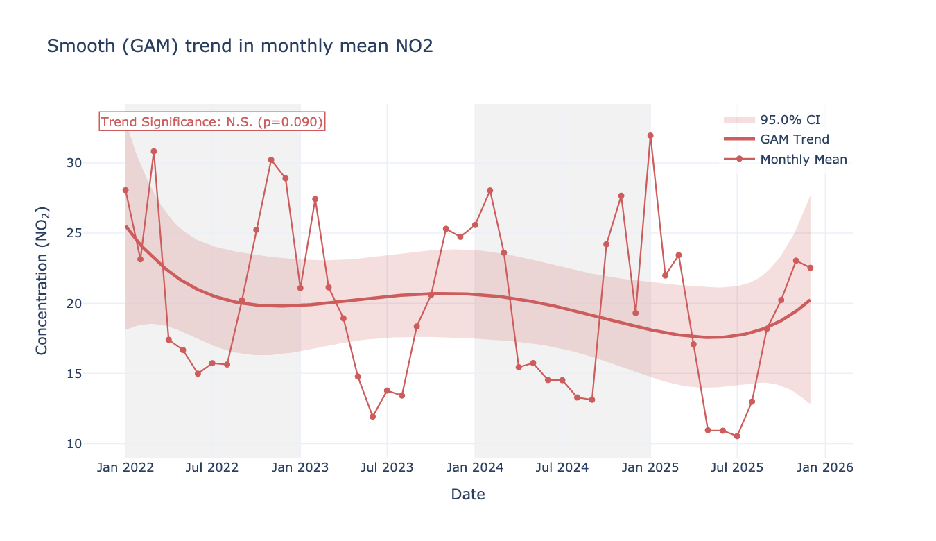
from PythonAQ import smooth_trend_plot

smooth_trend_plot(df, pollutant_col='NO2', avg_freq='MS').show()
time_plot
Time series for one or more pollutants, with optional grouping, stacking and normalisation.
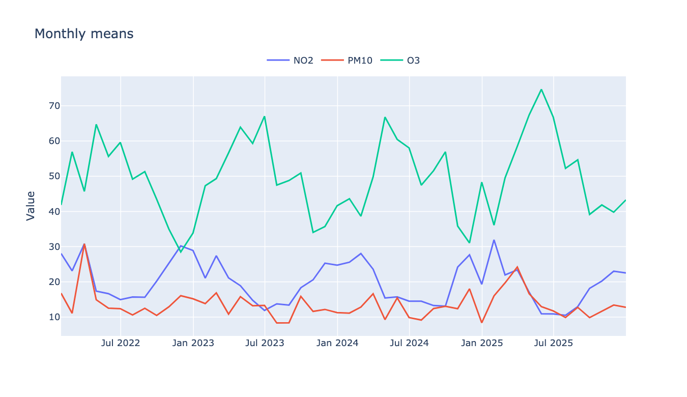
from PythonAQ import time_plot

time_plot(df, columns_to_plot=['NO2', 'PM10', 'O3'],
          averaging_period='ME', group_data=True).show()
trend_level
A heat map over two time dimensions, split into panels by a third.
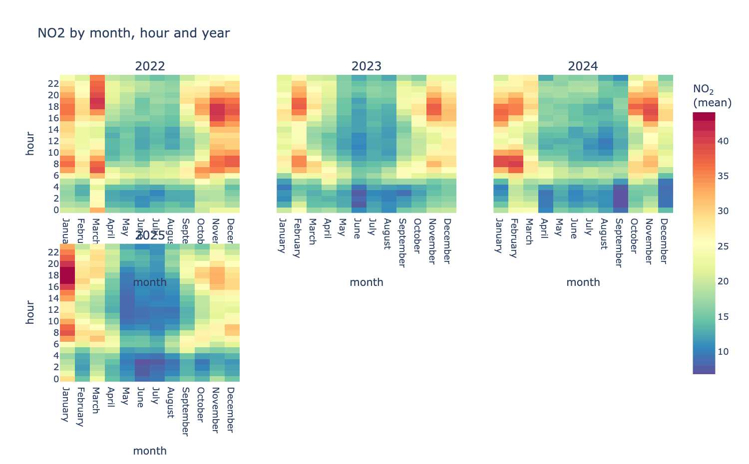
from PythonAQ import trend_level

fig, summary = trend_level(df, 'NO2', x='month', y='hour', type='year')
x,y(str): axes, from'hour','weekday','month','year','season','monthyear','wd', or any column.type(str or None): panel variable;Nonefor a single panel.statistic(str):'mean','median','max','min'or'frequency'.
time_prop
Stacked bars over time, split by the contribution of a category — the usual way source apportionment output is read.
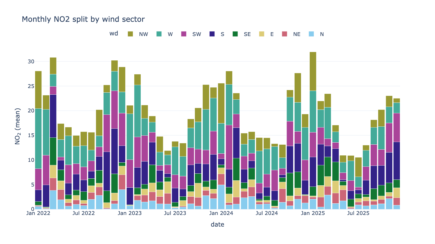
from PythonAQ import time_prop

fig, summary = time_prop(df, 'NO2', proportion='wd', avg_time='month')
proportion(str): the splitting column — an existing category, a numeric column split into quantiles, or anythingcut_dataunderstands.avg_time(str): bar width in time.statistic(str):'mean'or'sum'.normalise(bool): scale every bar to 100%, to compare composition rather than magnitude.
Segments are each category's share of the period, so the bars total the period statistic rather than summing category means.
calendar
Daily values as a calendar heat map. Needs the calendar extra.
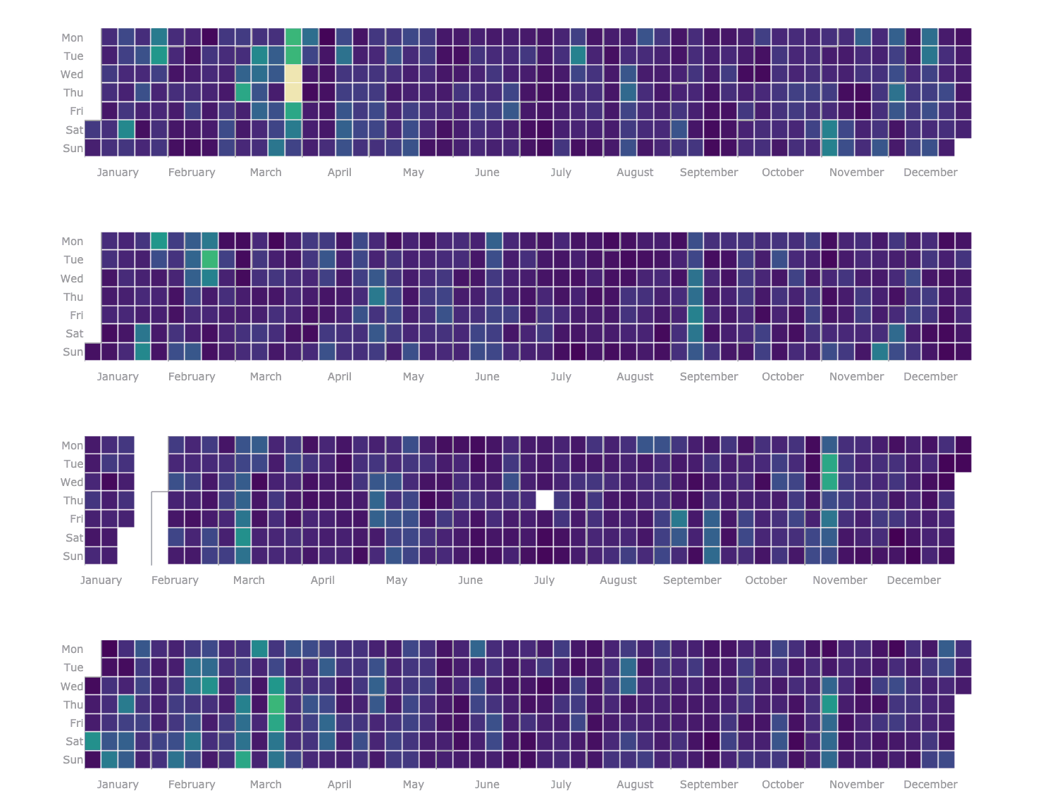
from PythonAQ import calendar

calendar(df, value_column='PM10').show()
Distributions and relationships
summary_plot
Time series, data-capture rug and histogram for every pollutant at once — the first thing to run on an unfamiliar dataset.
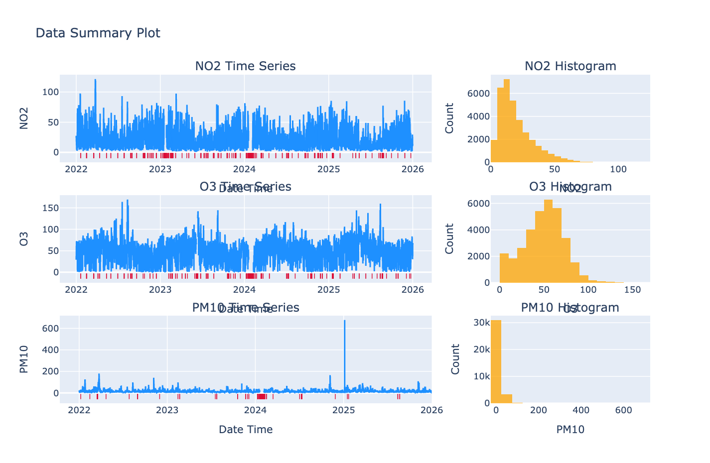
from PythonAQ import summary_plot

fig, summary = summary_plot(df[['date_time', 'NO2', 'PM10', 'O3']])
The summary DataFrame gives capture rate, missing count, min, max, mean,
median and 95th percentile per column.
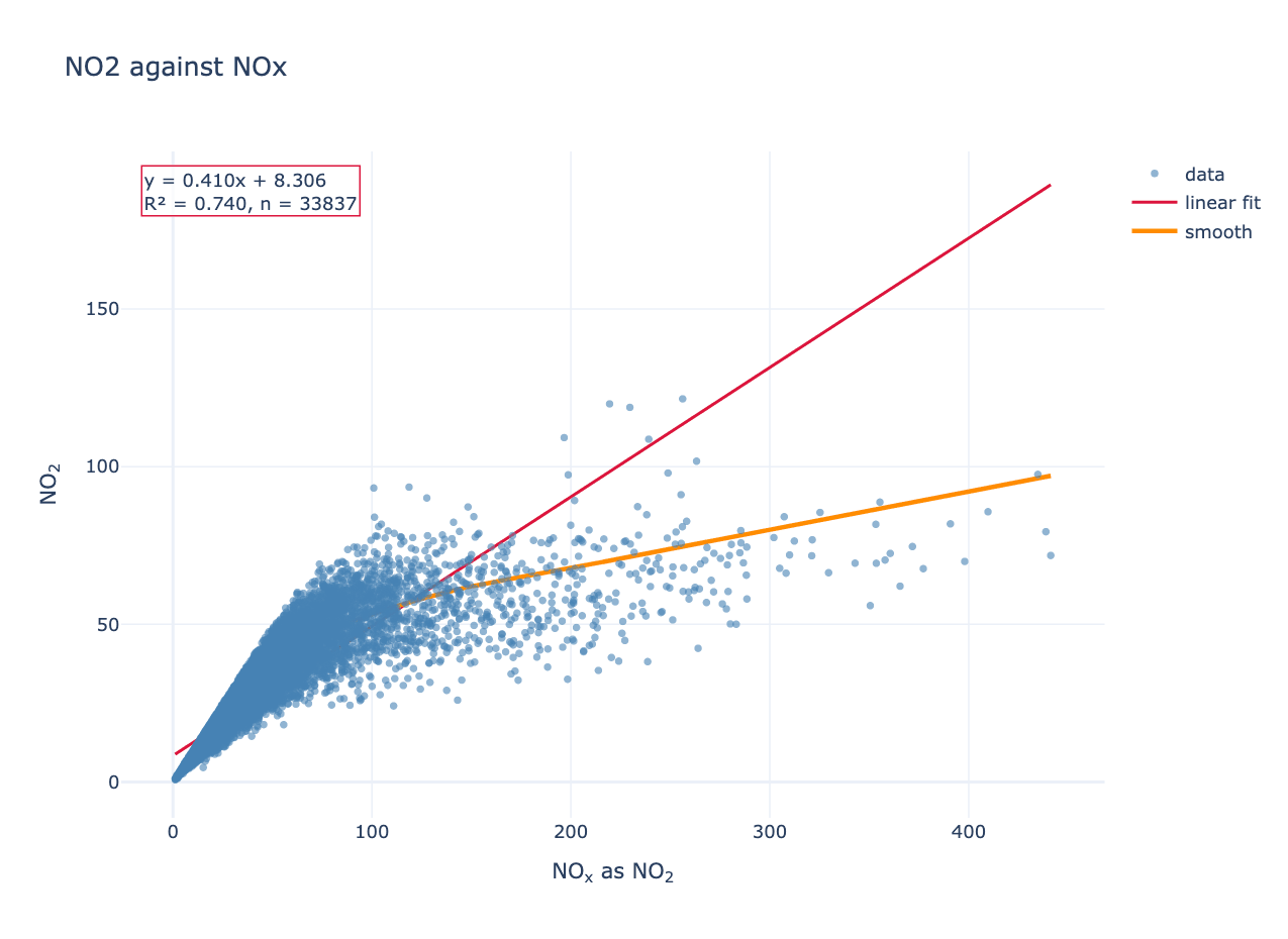
scatter_plot
Two variables against each other, with optional linear and LOWESS fits.
from PythonAQ import scatter_plot

fig, fit = scatter_plot(df, 'NOXasNO2', 'NO2', linear=True, smooth=True)
For Leeds Centre this gives NO₂ = 0.410 × NOₓ + 8.31, R² = 0.740. The slope below one and the curvature in the LOWESS fit reflect NO₂ making up a smaller share of NOₓ as total NOₓ rises, since the oxidant available to convert NO is limited.
method(str):'scatter','hexbin'or'density'.colour_by(str): column used to colour points.linear(bool),smooth(bool),one_to_one(bool): overlays.
Returns the figure and a DataFrame of fit statistics.
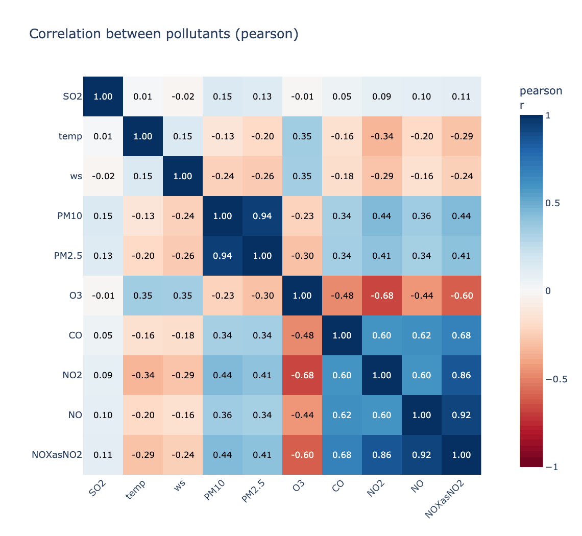
corr_plot
Correlation matrix, ordered by hierarchical clustering so related species sit together.
from PythonAQ import corr_plot

fig, corr = corr_plot(df, ['NO', 'NO2', 'NOXasNO2', 'O3', 'PM10', 'PM2.5'])
Strongest pair here is PM10/PM2.5 at r = 0.943; strongest anticorrelation is O₃ against NO₂ at r = −0.676.
method(str):'pearson','spearman'or'kendall'.cluster(bool),annotate(bool).
Model evaluation
mod_stats
Standard statistics for comparing modelled against observed values. The formulas follow the openair R source exactly, including the piecewise index of agreement of Willmott et al. (2011).
from PythonAQ import mod_stats

stats = mod_stats(df, mod='model', obs='observed', group_by='season')
Returns n, FAC2, MB, MGE, NMB, NMGE, RMSE, r, P, COE, IOA.
| Statistic | Meaning |
|---|---|
FAC2 |
Fraction of predictions within a factor of two |
MB, MGE |
Mean bias, mean gross error |
NMB, NMGE |
The same, normalised by the sum of observations |
RMSE |
Root mean square error |
r, P |
Pearson correlation and its p-value |
COE |
1 is perfect, 0 is no better than the observed mean, negative is worse |
IOA |
Index of agreement, −1 to +1 |
aq_stats
Annual summary statistics with exceedance counts against the UK objectives.
from PythonAQ import aq_stats

summary = aq_stats(df, 'NO2', data_thresh=75)
For Leeds Centre:
| year | data capture | mean | median | 95th pct | max daily | hours > 200 |
|---|---|---|---|---|---|---|
| 2022 | 97.6 | 22.2 | 18.3 | 50.5 | 66.5 | 0 |
| 2023 | 95.7 | 19.1 | 15.4 | 47.0 | 52.6 | 0 |
| 2024 | 93.7 | 19.2 | 15.8 | 45.6 | 49.0 | 0 |
| 2025 | 99.0 | 18.6 | 14.4 | 46.8 | 61.1 | 0 |
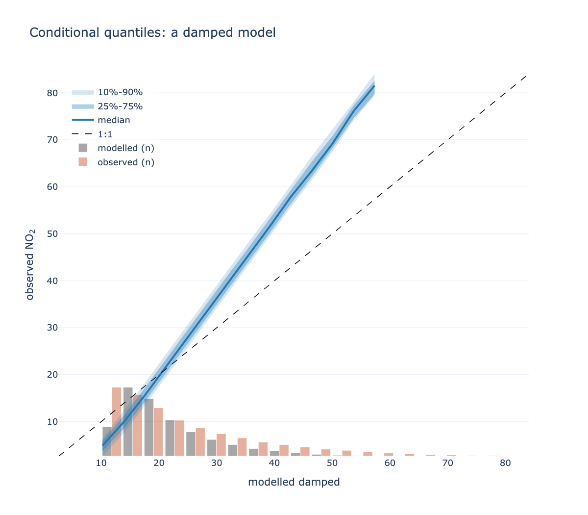
conditional_quantile
mod_stats says how well a model does; this says where it fails. Modelled
values are binned, and within each bin the spread of the corresponding
observations is drawn.
from PythonAQ import conditional_quantile

fig, summary = conditional_quantile(df, obs='observed', mod='model')
A model can have a respectable correlation while being badly wrong at high concentrations — the range that usually matters most — and that shows up here as the median peeling away from the 1:1 line at the top of the range.
bins(int or sequence): bins across the modelled range.min_count(int): bins with fewer pairs are dropped; a quantile of three points is not informative.quantiles(sequence): two nested pairs, default the 10/90 and 25/75.show_histograms(bool): the marginal distributions, which show where the data actually is — quantile bands alone say nothing about how many points support them.
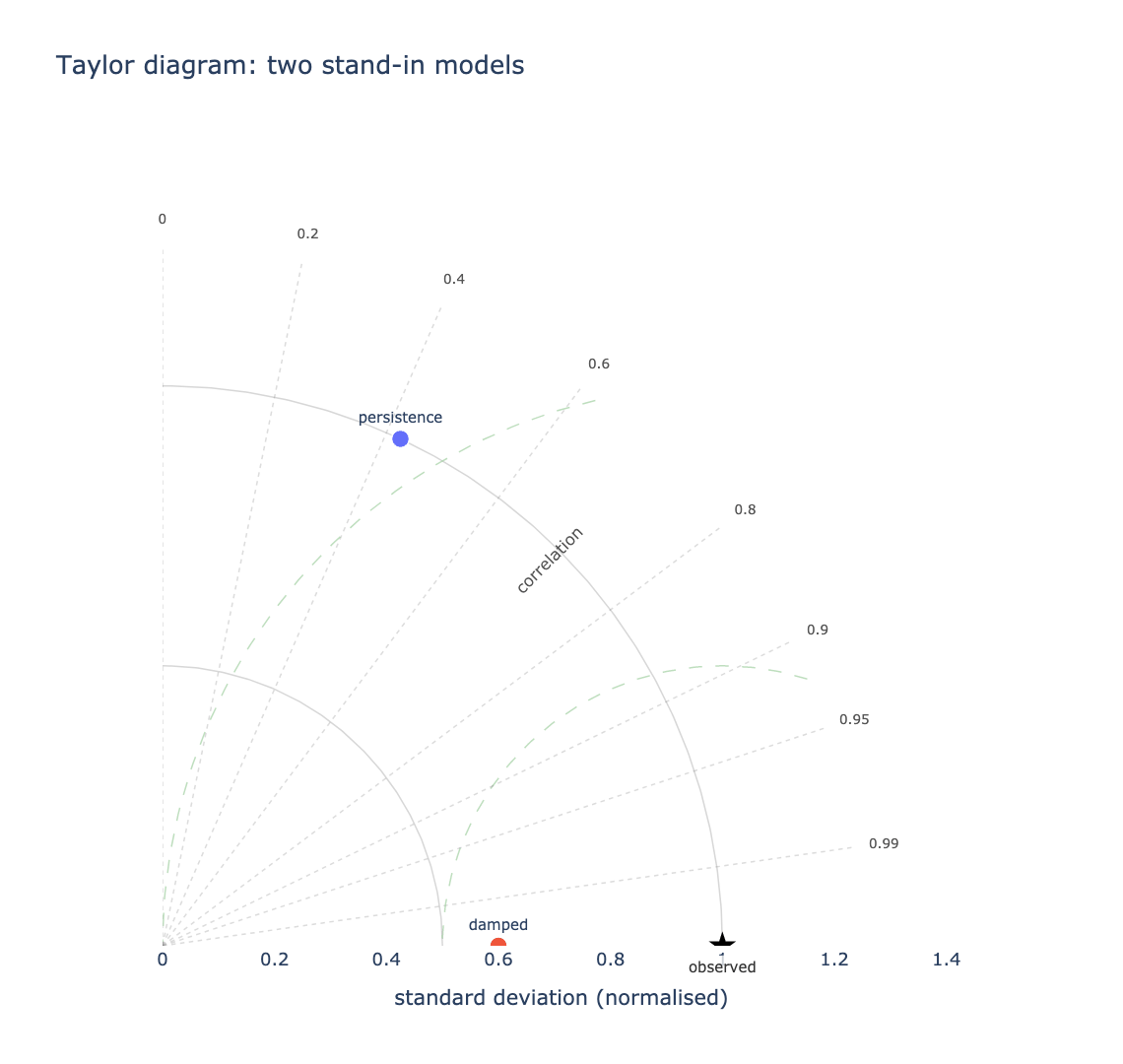
taylor_diagram
Three statistics on one plot. The radius is the standard deviation, the angle is the correlation, and — because of how those combine — the distance from a model's point to the reference point is its centred RMS error.
from PythonAQ import taylor_diagram

fig, summary = taylor_diagram(df, obs='observed', mod=['model_a', 'model_b'])
The closer a point sits to the star, the better the model. Comparing several becomes a matter of looking.
mod(str or list): one or several modelled columns.group(str or None): split the comparison, e.g. by season or site.normalise(bool): divide by the observed standard deviation, so series on different scales share one diagram.
Returns sd, r, centred_rmse and bias per point. Bias is reported
separately because the centred RMS error removes each series' mean by
construction — a model that is uniformly 20 µg/m³ too high has zero centred
error and sits exactly on the reference.
Data utilities
time_average
Average over a period, honouring a data-capture threshold.
from PythonAQ import time_average

daily = time_average(df, avg_time='day', data_thresh=75)
avg_time(str):'hour','day','3 day','month','year', or any pandas offset alias.data_thresh(float): minimum percentage of data required in a period; periods below becomeNaN.statistic(str):'mean','median','max','min','sum','sd','frequency','data.cap'or'percentile'.interval(str or None): the series' true sampling interval, e.g.'hour'. Only used whendata_threshis set.
Give
intervalwhen rows may be absent. Capture is measured against a regular time base, and inferring that base from the data uses the most common gap between observations — which is wrong exactly when data is missing. An hourly series with every other row absent looks like a complete two-hourly series and reports 100% capture on 50% of the data.date_paddoes the same job as a separate step.
Wind direction is averaged as a vector, not a scalar. Winds at 350° and 10° average to 0°, due north, rather than the 180° a naive mean would give. The scalar mean wind speed is kept; pass
vector_ws=Truefor the vector magnitude.
select_by_date
Subset by date components; all criteria combine with AND.
from PythonAQ import select_by_date

subset = select_by_date(df, year=2024, month='June', day=['Sat', 'Sun'])
winter = select_by_date(df, season='winter')
month takes names or numbers; day takes weekday names or month-days.
rolling_mean
Rolling mean with a data-capture threshold. The 8-point default matches the running 8-hour mean used for ozone.
from PythonAQ import rolling_mean

result = rolling_mean(df, 'O3', width=8, data_thresh=75)
align(str):'centre','left'or'right'.
cut_data
Add a conditioning column for splitting data.
from PythonAQ import cut_data

tagged = cut_data(df, type='season')
type(str):'year','month','monthyear','season','seasonyear','weekday','weekend','hour','daylight','wd', or a numeric column name (split inton_levelsquantiles).hemisphere(str):'northern'or'southern', for season definitions.
calc_percentile
Percentiles of a pollutant over a period.
from PythonAQ import calc_percentile

result = calc_percentile(df, 'NO2', percentile=[25, 50, 75, 95], avg_time='month')
date_pad
Pad a series onto a complete, regular time base.
from PythonAQ import date_pad

padded = date_pad(df, interval='hour')
Real monitoring data has gaps where rows are simply absent rather than
present-and-NaN, which quietly distorts anything that counts observations per
period. Give interval when that is possible: the base is otherwise inferred
from the most common gap between observations, which is wrong precisely when
data is missing. An hourly series with every other row absent looks like a
complete two-hourly series.
type(str or None): column identifying separate series, e.g.'site'. Each is padded over its own span, so a site that started reporting late does not gain years of empty rows.
split_by_date
Split a series at given dates.
from PythonAQ import split_by_date

result = split_by_date(df, '2023-06-01', labels=['before', 'after'])
N cut points give N+1 periods, as an ordered categorical — so it drops straight
into type= for before/after comparisons.
select_running
Find runs of consecutive values at or above a threshold.
from PythonAQ import select_running

episodes = select_running(df, 'NO2', run_length=8, mode='filter')
Episodes are defined by persistence rather than by any single high hour: one spike is not an episode, eight consecutive hours is. A gap ends a run rather than silently bridging it.
run_length(int),threshold(float or None, defaults to the 95th percentile),mode('flag'or'filter').
bin_data
Bin one variable against another, with bootstrap intervals on each bin.
from PythonAQ import bin_data

result = bin_data(df, x='ws', y='NO2', bins=20)
Answers "how does y behave across the range of x?" with an honest uncertainty per bin, rather than a single regression line that hides where the data is. Returns the bin centre, count, statistic, and lower and upper bounds.
deseason_data and get_period
Remove a seasonal cycle by decomposition.
from PythonAQ import deseason_data, get_period

ds = deseason_data(df, pollutant_column='NO2', interval='7D',
                   period=get_period('7D'), method='additive')
get_period converts a pandas interval string into the number of periods in a
year, which is what the decomposition needs.
Meteorological helpers
e_sat and rh
Saturation vapour pressure (hPa) and relative humidity (%).
from PythonAQ import e_sat, rh

e_sat(20.0)        # 23.34 hPa
rh(20.0, 10.0)     # 52.5 %
rh(15.0, 15.0)     # 100.0 %, saturated
Both take scalars or arrays. rh expects air temperature and dew point in °C
and clips the result to 0–100.
quick_text
Formats pollutant names and units for display. Applied automatically to the
titles, axis labels and colourbars of the plotting functions, so 'no2' on an
axis renders as NO₂.
from PythonAQ import quick_text

quick_text('no2')              # 'NO<sub>2</sub>'
quick_text('PM2.5 (ug/m3)')    # 'PM<sub>2.5</sub> (µg m<sup>-3</sup>)'
quick_text('Site 3 kerbside')  # unchanged
Matching is on whole tokens only. The species codes are short, so a careless
substring match would mangle ordinary prose — 'nothing', 'Nottingham' and
'concentration' all pass through untouched.
auto(bool): set False to disable, without branching at the call site.plain(bool): drop the markup, for contexts that do not render HTML.
Relationship to openair
PythonAQ follows openair using Python naming conventions — timeVariation
becomes time_variation. Where a statistic has a precise definition, such as
the modStats metrics, the formulas follow the openair R source exactly.
| openair | PythonAQ | openair | PythonAQ | |
|---|---|---|---|---|
importAURN etc. |
download_aurn_data |
timeAverage |
time_average |
|
importMeta |
import_aq_meta |
selectByDate |
select_by_date |
|
windRose |
wind_rose |
rollingMean |
rolling_mean |
|
pollutionRose |
pollutant_rose |
cutData |
cut_data |
|
percentileRose |
percentile_rose |
calcPercentile |
calc_percentile |
|
polarPlot |
polar_plot |
modStats |
mod_stats |
|
polarFreq |
polar_frequency_plot |
aqStats |
aq_stats |
|
polarCluster |
polar_cluster |
corPlot |
corr_plot |
|
timePlot |
time_plot |
scatterPlot |
scatter_plot |
|
timeVariation |
time_variation |
trendLevel |
trend_level |
|
TheilSen |
theil_sen_plot |
calendarPlot |
calendar |
|
smoothTrend |
smooth_trend_plot |
polarAnnulus |
polar_annulus |
|
quickText |
quick_text |
cutData / type |
type= everywhere |
|
conditionalQuantile |
conditional_quantile |
datePad |
date_pad |
|
TaylorDiagram |
taylor_diagram |
splitByDate |
split_by_date |
|
timeProp |
time_prop |
selectRunning |
select_running |
|
binData |
bin_data |
Not yet ported: polarDiff, conditionalEval, distPlot,
linearRelation, runRegression, the trajectory functions (trajPlot,
trajLevel, trajCluster), the remaining smoothers (GaussianSmooth,
WhittakerSmooth, kzFilter, rollingQuantile), and the openairmaps
interactive maps, which are a separate package.
Two deliberate differences:
time_averageaverages wind direction as a vector but keeps the scalar mean wind speed. Passvector_ws=Truefor the vector magnitude.cut_data(type='daylight')uses a fixed 07:00–19:00 window rather than openair's solar elevation calculation. Adequate for coarse splits; replace it before relying on it at high latitude or near the solstices.
Guide
docs/guide/index.html
is a single-page reference covering every public function, each with a short
example and the output that example actually produces — an interactive figure, a
table, or console output as appropriate.
Once Pages is enabled for the repository — Settings > Pages, source "GitHub Actions" — the workflow publishes it to chris-r-uol.github.io/PythonAQ/guide/. Until then, open the file locally or read it through the GitHub blob view.
It is generated by running the examples against real AURN data, so it cannot drift from the package:
pip install -e '.[calendar,docs]'
python examples/build_guide.py
The page has light, dark and system themes. Figures are embedded as Plotly JSON
rather than images so they restyle live rather than needing two PNGs each, and
the site map follows suit — carto-positron in light, carto-darkmatter in
dark. Both are OpenStreetMap data rendered muted, so the markers stay readable
against them.
The build asserts its own coverage and exits non-zero if a public function is left undocumented.
Worked example
examples/demo_leeds.py runs every public
function against real data for Leeds Centre and writes each figure to
examples/output/ as standalone interactive HTML:
pip install -e '.[calendar]'
python examples/demo_leeds.py
It downloads ~35,000 hourly records plus meteorology from the nearest NOAA
station, caches them so re-runs are instant, and checks its own coverage —
exiting non-zero if any public function goes unexercised. Pass --refresh to
re-download.
Streamlit application
pip install -e '.[app,calendar]'
streamlit run app.py
Development
pip install -e '.[dev]'
pytest
The tests use synthetic data throughout and never touch the network, so they run offline and deterministically. CI covers Python 3.9–3.14 on Linux, plus macOS and Windows.
To rebuild the figures in this manual after changing a plotting function:
pip install -e '.[calendar,docs]'
python examples/build_readme_figures.py
Releasing
Publishing is automated but deliberately gated. It happens when a GitHub release is created, never on an ordinary push.
# 1. bump the version (one source of truth)
#    PythonAQ/__init__.py  ->  __version__ = "0.5.1"
# 2. merge, tag and release
git tag -a v0.5.1 -m "PythonAQ 0.5.1"
git push origin v0.5.1
gh release create v0.5.1 --title "PythonAQ 0.5.1" --notes-from-tag --verify-tag --latest
The Publish workflow then builds an sdist and a wheel, runs twine check,
verifies the tag matches the packaged version, installs from the sdist to
prove it is complete, and uploads to PyPI.
Uploads use Trusted Publishing: PyPI verifies a short-lived OpenID Connect token minted by GitHub for this specific repository, workflow and environment, and issues an upload token in return. No API token is stored in the repository, so there is no secret to leak or rotate.
One-time setup
On PyPI — add a trusted publisher at pypi.org/manage/account/publishing (for a project that does not exist yet) or the project's Publishing settings:
| Field | Value |
|---|---|
| Owner | chris-r-uol |
| Repository | PythonAQ |
| Workflow name | publish.yml |
| Environment | pypi |
In this repository — create the environment under Settings → Environments
named pypi. Adding a required reviewer there means a release waits for an
explicit approval before anything uploads, which is worth having: a PyPI
version number can never be reused, even after deletion.
Rehearsing
Repeat both steps on test.pypi.org with the
environment named testpypi, then run the workflow manually:
gh workflow run publish.yml -f target=testpypi
That path uses skip-existing, so repeated rehearsals do not fail.
Contributing
Contributions are welcome — please open an issue or pull request.
Licence
MIT. See LICENSE.
1 maintainer

Metadata
1 maintainer
Release files for PythonAQ 0.5.1
For a detailed explanation of source distributions (sdists) and built distributions (wheels), please see the package formats documentation.
Source distribution (sdist)
| File | Size | Uploaded | |
|---|---|---|---|
| pythonaq-0.5.1.tar.gz | 133.2 kB | Details |
Built distribution (wheel)
| File | Interpreter | ABI | Platform | Reset |
|---|---|---|---|---|
| pythonaq-0.5.1-py3-none-any.whl | Python 3 | none | any | Details |
Total release size: 235.6 kB
Release files / pythonaq-0.5.1.tar.gz
| Download URL | pythonaq-0.5.1.tar.gz |
|---|---|
| Size | 133.2 kB |
| Tags | Source |
|
SHA-256 checksum How to use checksums |
7ab8dffcbc15ebae9bf9c98b87294f051d0cc73fe42a66c9328208a230fb714c
|
|
BLAKE2b-256 checksum How to use checksums |
7edd0b1658c57dcf150b3a06a6d8ce1dbe91cf2d4b39a9b8b4f410c92810dc92
|
| Upload date | |
|
Uploaded using Trusted Publishing? What is trusted publishing? |
Yes |
| Uploaded via |
twine/7.0.0 CPython/3.13.14
|
Provenance
Provenance describes where a file came from. On PyPI, provenance is shared via attestations, which provide a verifiable record of the build or publishing details. View details, limitations and caveats.


PyPI Publish Attestation
PyPI verified that this artifact, at this checksum, originated from the publisher listed below.
Signed by GitHub Actions, verified by PyPI on Aug 17, 2026.
Transparency logRelease files / pythonaq-0.5.1-py3-none-any.whl
| Download URL | pythonaq-0.5.1-py3-none-any.whl |
|---|---|
| Size | 102.4 kB |
| Tags | Python 3 |
|
SHA-256 checksum How to use checksums |
ffea033a933cfb4dc2ed27cf1bef4d2f6713708d2093d3481eb4798309ff059b
|
|
BLAKE2b-256 checksum How to use checksums |
3d1a69ebaf54ec4f109a2dccf30356d70313eee1f63d913d1e38e00e41d8ca72
|
| Upload date | |
|
Uploaded using Trusted Publishing? What is trusted publishing? |
Yes |
| Uploaded via |
twine/7.0.0 CPython/3.13.14
|
Provenance
Provenance describes where a file came from. On PyPI, provenance is shared via attestations, which provide a verifiable record of the build or publishing details. View details, limitations and caveats.
PyPI Publish Attestation
PyPI verified that this artifact, at this checksum, originated from the publisher listed below.
Signed by GitHub Actions, verified by PyPI on Aug 17, 2026.
Transparency log












