QtSLIX is an expansion to the Scattered Light Imaging ToolboX by adding a graphical user interface.

Project description
QtSLIX -- A graphical user interface for the Scattered Light Imaging ToolboX
Introduction
Scattered Light Imaging (SLI) is a novel neuroimaging technique that allows to explore the substructure of nerve fibers, especially in regions with crossing nerve fibers, in whole brain sections with micrometer resolution (Menzel et al. (2020)). By illuminating histological brain sections from different angles and measuring the transmitted light under normal incidence, characteristic light intensity profiles (SLI profiles) can be obtained which provide crucial information such as the directions of crossing nerve fibers in each measured image pixel.
To analyze the Scattered Light Imaging measurements, a toolbox named Scattered Light Imaging ToolboX (SLIX) was implemented – an open-source Python package that allows a fully automated evaluation of SLI measurements and the generation of different parameter maps. The purpose of SLIX is twofold: First, it allows to transform the raw data of SLI measurements (SLI image stack) to human-readable parameter maps that can be used for further analysis and interpreted by researchers. To this end, SLIX also contains functions to visualize the resulting parameter maps, e.g. as colored vector maps. Second, the results of SLIX can be processed further for use in tractography algorithms. For example, the resulting fiber direction maps can be stored as angles or as unit vectors, which can be used as input for streamline tractography algorithms (Nolden et al. (2019)).
However, not everyone is familiar with the command line or the Python programming language and might not be able to use SLIX. This package is designed to be used as a graphical user interface only allowing users unfamiliar with the command line to easily perform the necessary steps to analyze SLI measurements. Almost all available options of the command line are also available in the graphical user interface. Users are able to run the analysis pipeline, visualize their results and cluster the parameter maps.
Install instructions
Requirements
QtSLIX requires the following packages:
- Python 3.6 or higher
- PyQt5
- NumPy
- SLIX v2.4.0 or higher
- Matplotlib
SLIX itself requires the following packages:
- Python 3.6 or higher
- Tifffile
- Nibabel
- h5py
- Pillow
- Numba
- Matplotlib
- tqdm
- SciPy
- Imagecodecs
To use GPU acceleration, SLIX requires the following packages:
- CuPy >= v8.0.0
It is advised to use a system with the following minimal requirements:
- Operating System: Windows, Linux, MacOS
- Python version: Python 3.6+
- Processor: At least four threads if executed on CPU only
- RAM: 8 GiB or more
- (optional GPU: NVIDIA GPU supported by CUDA 9.0+)
Installation of QtSLIX
How to clone QtSLIX (for further work)
git clone git@github.com:3d-pli/QtSLIX.git
cd QtSLIX

# A virtual environment is recommended:
python3 -m venv venv
source venv/bin/activate

pip3 install -r requirements.txt
How to install QtSLIX as Python package
# Install via PyPi
pip install QtSLIX

# Install after cloning locally
git clone git@github.com:3d-pli/QtSLIX.git
cd QtSLIX
pip install .
Run QtSLIX locally
git clone git@github.com:3d-pli/QtSLIX.git
cd QtSLIX
python3 bin/main.py

# alternatively, after installation of SLIX
pip3 install QtSLIX
QtSLIX
Running the application
Starting the application
To start the application, just run the following command in a command line interface:
# If you installed QtSLIX as a Python package:
QtSLIX

# Else, if you installed QtSLIX locally:
python3 bin/main.py
General interface
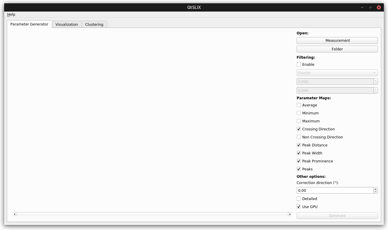
When opening the program for the first time, you will be greeted with the interface shown in the figure above. The menu bar only contains a help option where things like the license and a link to the repository are stored.
Below that menu bar, a list of available analysis steps is shown. The application will always start in the
Parameter Generator tab. In the following, we will only discuss the available tabs with their functions.
Parameter Generator
The Parameter Generator tab allows you to generate parameter maps for the analysis of SLI measurements.
The available options mostly match those of the command line program SLIXParameterGenerator which gets installed
when you install the package SLIX. You can see the command line options here.
The left area is a preview window of a loaded measurement. When using one of the buttons Measurement or Folder, you will be able to open a SLI measurement.
The preview window will then show the loaded measurement as seen below.
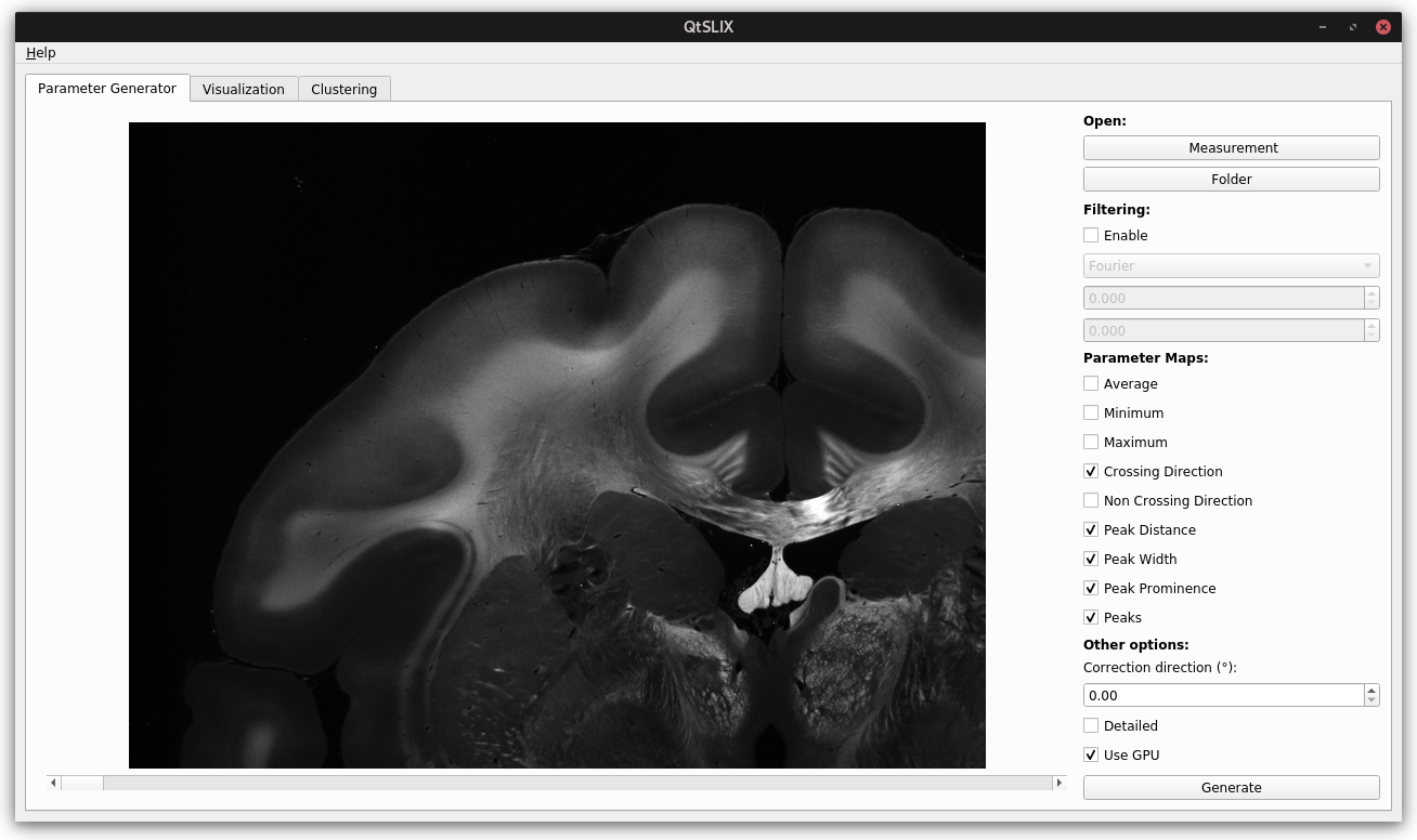
There is a scroll bar below the measurement which can be used to scroll through all the measurement angles. This way, one can ensure that the correct measurement is loaded and no image contains wrong information.
The right side then allows to select the parameters that should be generated. If a measurement with an angular step size other than 15° is loaded, it might be helpful to enable the Filtering option. When enabled, you are able to choose between the Fourier and Savitzky-Golay filters. The two number fields allow you to choose the window size and the polynomial order for the Savitzky-Golay filter or the cutoff frequency and smoothing for the Fourier filter.
The Parameter Maps section contains a number of check boxes which allow you to select which parameters should be generated. The resulting parameter maps are explained in detail in the SLIX repository. You can find the explanation here.
The other option section contains a number of options that are not directly related to the parameter generation. For example, you can choose a correction angle for the direction which will change the resulting direction angle. Enabling the detailed option will result in 3D images of some parameter maps which might be helpful for further analysis. The Use GPU option will enable the use of a GPU for the calculation of the parameter maps. This might be helpful if you have a GPU and you want to speed up the calculation. However, the calculations are pretty memory intensive. Therefore, the program might throw an error message if the memory is not sufficient.
Click on the Generate button to generate the parameter maps. A save dialog will open where you can choose where to save the parameter maps.
The file names are generated based on the input file name / input folder name. The extension of the file is automatically added and defaults to .tiff in the current version.
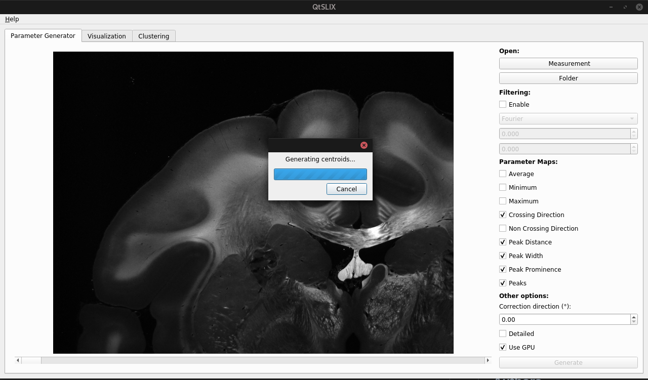
A progress bar will show the progress of the calculation. You are able to use the graphical user interface in the meantime.
Visualization
The second available tab in the interface covers the visualization of resulting parameter maps. The general interface can be seen below.
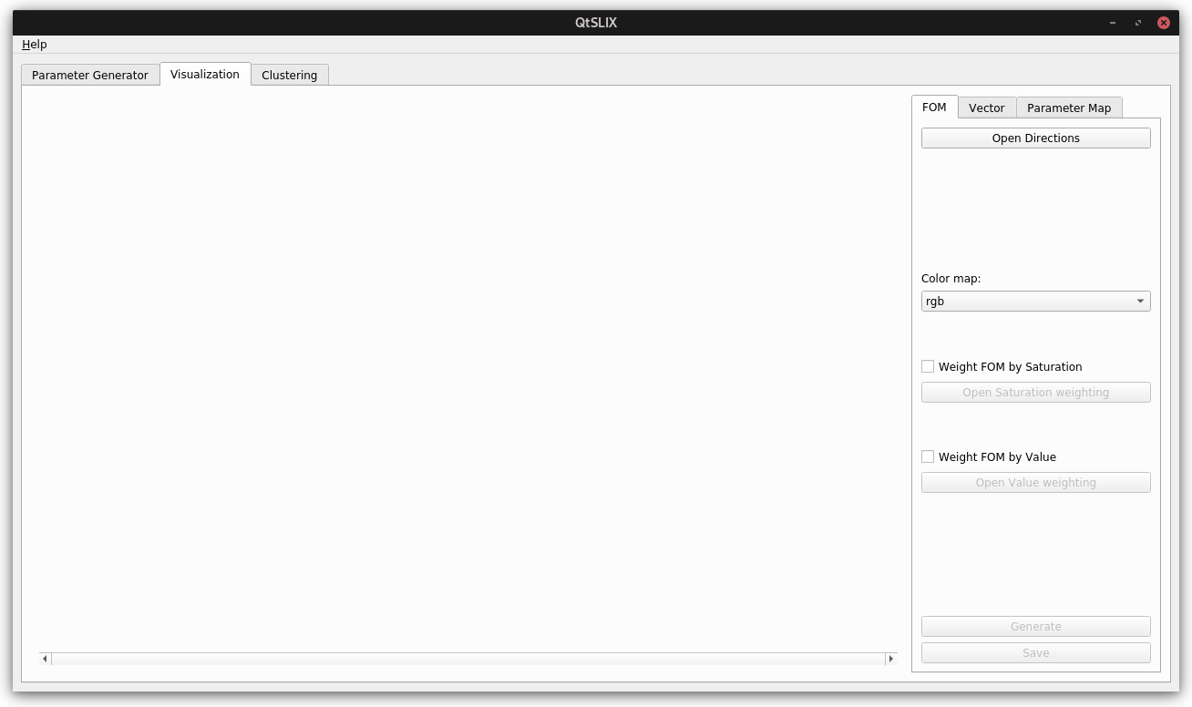
The right side has three options to visualize or show parameter maps:
- FOM: Visualize up to four direction maps as a fiber orientation map
- Vector: Visualize the direction maps as unit vectors on top of an SLI measurement or parameter map
- Parameter Map: Visualize the parameter maps as a color map
FOM
A fiber orientation map is a map of the direction of the fibers in the image. Each pixel gets assigned a color based on the direction and inclination angle of the fibers in the underlying image. This method for visualizing fiber orientation maps is described in this paper. A direct example can be found here. There are different ways to visualize the direction maps. QtSLIX supports all implemented variants offered by SLIX. For the available SLIX options, look here.
When clicking on Open Directions, a dialog will open where you can choose the direction maps to visualize. After choosing the files, you can choose between the following color maps:
- RGB: The direction is visualized as a red, green and blue color. The red and green channel are used for the in-plane direction. The blue channel is used for the inclination angle.
- HSVBlack: The direction color is visualized as the hue of the HSV color space. The saturation is set to 1 and the value is determined by the inclination angle.
- HSVWhite: The direction color is visualized as the hue of the HSV color space. The saturation is determined by the inclination angle and the value is set to 1.
- HSVBlack_r: Same as HSVBlack. However, the direction angle is flipped (180° - dir).
- HSVWhite_r: Same as HSVWhite. However, the direction angle is flipped (180° - dir).
Both the saturation and value channel can also be used to weight the generated color map. If you want to use the saturation channel, you can use the checkmark next to Weight FOM by Saturation and load a parameter map which will be used for weighting. The parameter map will get normalized to a range of 0-1 to ensure that the color map is in the correct range. The same procedure holds true for the value channel.
Clicking on the Generate button will generate the FOM and show a preview on the left side of the interface. This might take a while depending on the image size. The graphical user interface will freeze during the calculation.
After the calculation is finished, the result can also be saved using the Save button. The button is grayed out until at least a preview was generated. Using the Save option will open a save dialog where you can choose where to save the FOM. Both the .tiff and .h5 file format are supported.
Vector
Similar to the fiber orientation map, vectors can be used to visualize the direction maps on top of an SLI measurement or parameter map. The vectors will be shown as lines with a defined with and length. The color of the lines is determined by the direction angles and will follow the color spaces of the fiber orientation map. The general interface can be seen below.
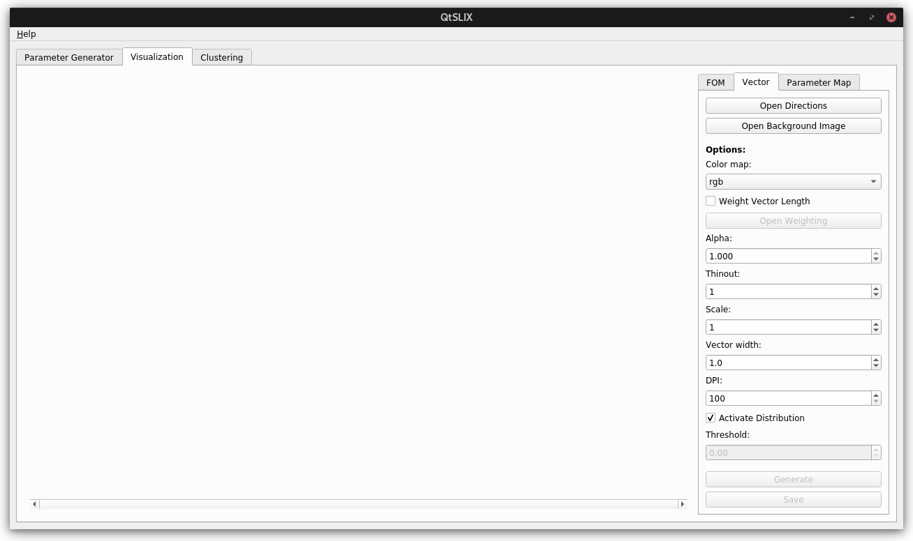
Here the background image can be loaded by clicking on the Open Background Image button. In addition, the vector length can be weighted by using a parameter map which will be normalized to a range of 0-1.
Parameters like Alpha or Thinout will be used to control the appearance of the vector and will result in the same results you expect when using the command line options of SLIX.
| Argument | Function |
|---|---|
Alpha |
Factor for the vectors which will be used during visualization. A higher value means that the vectors will be more visible. (Value range: 0 -- 1) |
Thinout |
Thin out vectors by an integer value. A thinout of 20 means that both the x-axis and y-axis are thinned by a value of 20. Default = 20 |
Scale |
Increases the scale of the vectors. A higher scale means that the vectors in the resulting image are longer. This can be helpful if many pixels of the input image are empty but you don't want to use the thinout option to see results. If the scale option isn't used, the vectors are scaled by the thinout option. |
Vector width |
Change the default vector width shown in the resulting image. This can be useful if only a small number of vectors will be shown (for example when using a large thinout) |
Threshold |
When using the thinout option, you might not want to get a vector for a lonely vector in the base image. This parameter defines a threshold for the allowed percentage of background pixels to be present. If more pixels than the threshold are background pixels, no vector will be shown. (Value range: 0 -- 1) |
Dpi |
Set the image DPI value for Matplotlib. Smaller values will result in a lower resolution image which will be written faster. Larger values will need more computation time but will result in clearer images. Default = 1000dpi |
Distribution |
Instead of using each n-th vector for the visualization (determined by the median vector), instead show all vectors on top of each other. Note: Low alpha values (around 1/alpha) are recommended. The threshold parameter is disabled when enabling the distribution. |
Like with the FOM, clicking on Generate will generate the vector image and show a preview of the result. Please keep in mind that the calculation of the vector image can take a while, especially when using the distribution option. The graphical user interface will freeze in the meantime.
Using the Save option will open a save dialog where you can choose where to save the FOM. Both the .tiff and .h5 file format are supported.
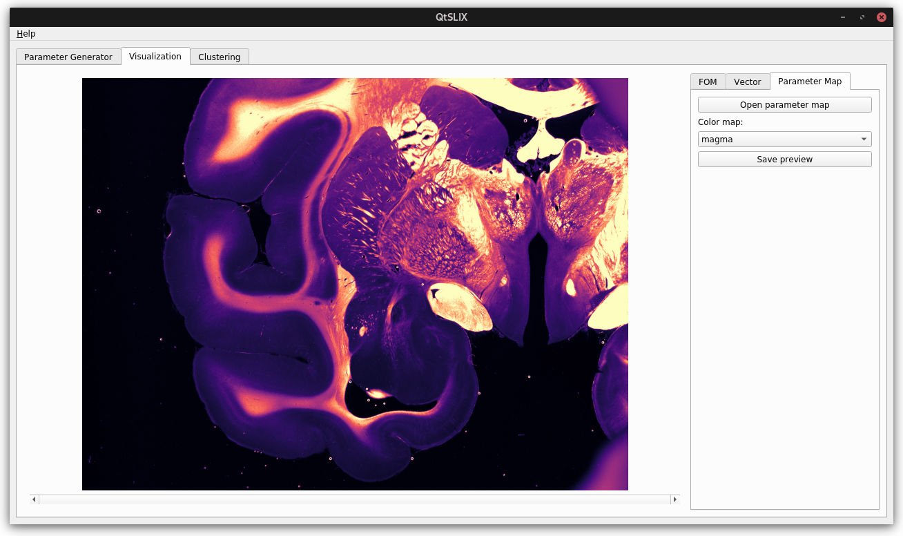
Parameter map
The last available tab contains the simple visualization of parameter maps. The user is able to load a parameter map using the ... option. Loading a parameter map automatically shows it on the left side in the image preview. Using a drop-down menu, the user can select Matplotlib color space used for the visualization. The user is then able to save to colorized parameter map using the Save preview option.
Currently, there is no support for a colorized legend next to the parameter map. This feature may be explored in the future.
A preview of the view is shown below.
Clustering
The last available tab contains the clustering of a measurement based on the generated parameter maps.
Keep in mind that, just like with the normal version of SLIXCluster, optional parameter maps like Min and Max
might be required to ensure that all clustering steps can function as expected.
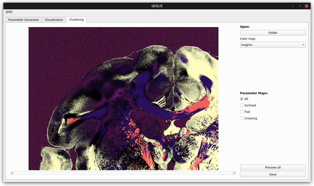
Clicking on the Folder option will open a folder selection dialog. Here, all needed files need to be located. Just like in the parameter map, the user can select the Matplotlib color space used for the visualization.
Using the four checkboxes below, the user can select which classification masks shall be generated. Unlike the preview, the results will not be colorized and will instead be saved as an 8-bit image where each number corresponds to a classification. For more information which classification numbers correspond to which masks, please refer to the SLIXCluster documentation
Clicking on Save will generate and save all checked masks. The user can select the folder where all files will be saved. The filenames will be based on the parameter map names.
Authors
- Jan André Reuter
References
 |
Fiber Architecture - INM1 - Forschungszentrum Jülich |
 |
Human Brain Project |
Acknowledgements
This open source software code was developed in part or in whole in the Human Brain Project, funded from the European Union’s Horizon 2020 Framework Programme for Research and Innovation under the Specific Grant Agreement No. 785907 and 945539 ("Human Brain Project" SGA2 and SGA3). The project also received funding from the Helmholtz Association port-folio theme "Supercomputing and Modeling for the Human Brain".
License
This software is released under MIT License
Copyright (c) 2021-2022 Forschungszentrum Jülich / Jan André Reuter.

Permission is hereby granted, free of charge, to any person obtaining a copy of this software and associated documentation files (the "Software"), to deal in the Software without restriction, including without limitation the rights to use, copy, modify, merge, publish, distribute, sublicense, and/or sell copies of the Software, and to permit persons to whom the Software is furnished to do so, subject to the following conditions:

The above copyright notice and this permission notice shall be included in all copies or substantial portions of the Software.python input parameters -i -o

THE SOFTWARE IS PROVIDED "AS IS", WITHOUT WARRANTY OF ANY KIND, EXPRESS OR IMPLIED, INCLUDING BUT NOT LIMITED TO THE WARRANTIES OF MERCHANTABILITY, FITNESS FOR A PARTICULAR PURPOSE AND NONINFRINGEMENT. IN NO EVENT SHALL THE AUTHORS OR COPYRIGHT HOLDERS BE LIABLE FOR ANY CLAIM, DAMAGES OR OTHER LIABILITY, WHETHER IN AN ACTION OF CONTRACT, TORT OR OTHERWISE, ARISING FROM, OUT OF OR IN CONNECTION WITH THE SOFTWARE OR THE USE OR OTHER DEALINGS IN THE SOFTWARE.
Release history Release notifications | RSS feed


Download files
Download the file for your platform. If you're not sure which to choose, learn more about installing packages.
Source Distribution
Built Distribution
Filter files by name, interpreter, ABI, and platform.
If you're not sure about the file name format, learn more about wheel file names.
Copy a direct link to the current filters
File details
Details for the file QtSLIX-1.0.2.tar.gz.
File metadata
- Download URL: QtSLIX-1.0.2.tar.gz
- Upload date:
- Size: 35.5 kB
- Tags: Source
- Uploaded using Trusted Publishing? No
- Uploaded via: twine/3.7.1 importlib_metadata/4.10.1 pkginfo/1.8.2 requests/2.27.1 requests-toolbelt/0.9.1 tqdm/4.62.3 CPython/3.9.10
File hashes
| Algorithm | Hash digest | |
|---|---|---|
| SHA256 |
476955f8ab1bf6e8ca0a9d17678aff4f30559e0aff0863a730bc7cf06b78c290
|
|
| MD5 |
d36c3a8ec250175d62117b6e49959f14
|
|
| BLAKE2b-256 |
8edf715e7016f0e82a7a67a367250359c77f45704015d565d349f4266b0be16f
|
File details
Details for the file QtSLIX-1.0.2-py3-none-any.whl.
File metadata
- Download URL: QtSLIX-1.0.2-py3-none-any.whl
- Upload date:
- Size: 27.8 kB
- Tags: Python 3
- Uploaded using Trusted Publishing? No
- Uploaded via: twine/3.7.1 importlib_metadata/4.10.1 pkginfo/1.8.2 requests/2.27.1 requests-toolbelt/0.9.1 tqdm/4.62.3 CPython/3.9.10
File hashes
| Algorithm | Hash digest | |
|---|---|---|
| SHA256 |
3473a03b53f09b714eb9d5734c5f5519ad28e63faafc7b7b5f7209c21ea9acc3
|
|
| MD5 |
82145f916ec8168b4d17baffb537cb81
|
|
| BLAKE2b-256 |
17caf82445aa777c77f0bdbcb40e70ce8141520d375a0057589490ea70aa6b10
|


