package for quantify early-stage LUAD progression from CT image

Project description
RadioTrace
RadioTrace is a Python package to quantify and visualize the progression status of early-stage lung adenocarcinoma (esLUAD) from CT images. It is designed and developed by Jiaqi Li from XGlab, Tsinghua University. The work is collaborated with Prof. Wenzhao Zhong's group from Guangdong Provincial People's Hospital and Prof. Lin Yang's group from Shenzhen People's Hospital.
RadioTrace package is free for academic use. Please contact the authors for commercial usage.
Install
The RadioTrace package integrates the use of Python and R. Don't worry, we have wrapped the R functions in the Python code and users only need to install some packages and then write Python code only.
BTW, consider the potential conflicts of packages, we strongly suggest you to install the packages in a new anaconda environment :)
First let's install the python packages. Please pay special attention to PyTorch if you want to use GPU. It is easy to download the proper version of GPU version PyTorch from the official webpage (https://pytorch.org/get-started/locally/). In this case, make sure that you install the GPU version PyTorch before install RadioTrace.
After that, or if you only need CPU version PyTorch, install RadioTrace packages.
pip install radiotrace
Next, let's install the R packages. We also install the R using anaconda:
conda install -c conda-forge r-base
Then enter the R programming software by one character of code:
R
The R package we need is the slingshot (Street et al., BMC Genomics, 2018), which can be installed from Bioconductor. Here we use two lines of code to install these two packages:
install.packages("BiocManager")
BiocManager::install("slingshot")
Now we have finished package installation. It's time to explore the use of RadioTrace.
Tutorial
By running RadioTrace package users are walking through several steps: Load image and segmentation, Locate and extract tumor, Load projection functions, Inference the emebedding vector(s) and coordinate(s) in PCA space, Visualization and Quantify progression status. Here we did clustering on the pixel-wise radiomic features.
0. Load packages
import os
import numpy as np
import matplotlib.pyplot as plt

from radiotrace.load import load_image, load_seg
from radiotrace.locate import locate_tumor
from radiotrace.get_projection import get_model, get_pca
from radiotrace.inference import model_inference, pca_trans
from radiotrace.visualize import visualize_reference, visualize
from radiotrace.calPPS import calPPS
from radiotrace.utils import cal_tumor_size, get_largest_slice
1. Load image and segmentation
Here we use public NSCLC-RadioGenomics data as an example. This is a public dataset available on The Cancer Imaging Archive (TCIA). Here the image and segmentation are stored in the NIFTI (.nii.gz) format.
dicom_path = "./RadioGenomics/R01-001_img.nii.gz"
seg_path = "./RadioGenomics/R01-001_seg.nii.gz"
image = load_image(dicom_path)
seg = load_seg(seg_path)
print(image.shape, seg.shape)
(304, 512, 512) (304, 512, 512)
2. Locate and extract tumor
Next, we locate the tumor using segmentation mask, and extract the tumor image with bounding box.
tumor_image, tumor_mask = locate_tumor(image, seg)
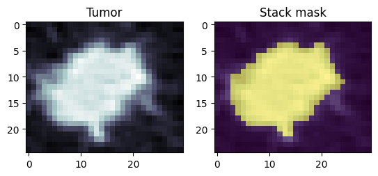
We can visualize a slice of the extracted tumor corresponding mask.
img2d, mask2d = get_largest_slice(tumor_image, tumor_mask)
plt.subplot(121)
plt.imshow(img2d, cmap="bone")
plt.title("Tumor")
plt.subplot(122)
plt.imshow(img2d, cmap="bone")
plt.imshow(mask2d, alpha=0.5)
plt.title("Stack mask")
3. Prepare data and load projection functions
We use a deep learning model and a PCA transform function to project the tumor image to the PCA space of training set. Here we prepare the tumor image data for model input and then load the projection functions.
If you want to use GPU to do the inference, remember to specify the environment variable before loading the model.
You will need some files such as pre-trained weights, transformation functions, etc. We have wrapped them into the package and please keep the paths unchanged. These files are also available on GitHub: https://github.com/LiJiaqi96/RadioTrace.
size = [cal_tumor_size(tumor_mask)]
tumor_image = [tumor_image]

## Optional: specify GPU device
# os.environ['CUDA_VISIBLE_DEVICES'] = '1'

model = get_model("./data/cnn_proj_weights.pkl")
pca_func = get_pca("./data/pca_trans.sav")
Note that the input image should be in shape (N Z H W), and tumor size should be a list. Here we show the example of inference one tumor. Just append more samples to the list if you want to inference multiple samples.
4. Project the tumor image to vectors
In this step, we will project the tumor image to the embedding vectors, then to the PCA spacce of training set. It will not take a long time when using CPU and it is very easy to switch between CPU and GPU mode using the argument "use_GPU".
pred_embed = model_inference(tumor_image, size, model, use_GPU=False)
pca_embed = pca_trans(pred_embed, pca_func)
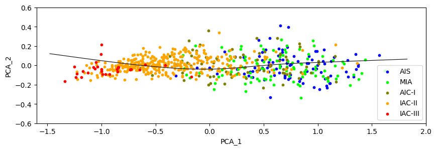
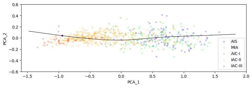
5. Visualize the progression status of the inference tumor
We provide two visualization functions for users to visualize the reference trajectory and samples in the training set, as well as the relative position of the inference tumors.
## Visualize the reference only
fig = visualize_reference(reference_data_path="./data/ref_data.json", curve_data_path="./data/curve_data.npy")
## Visualize the reference and inference tumors. Use "transparency" argument to adjust the color of training samples.
fig = visualize(reference_data_path="./data/ref_data.json", curve_data_path="./data/curve_data.npy", transparency=0.2)
6. Calculate pseudo-progression score (PPS)
Finally, we quantify the progression status of the inference tumor(s). The PPS=0 indicates the earliest progression status. This step will return a list of PPS values.
pps = calPPS(pca_embed, reference_data_path="./data/ref_data.json", traj_obj_path="./data/traj_obj.rds")
[2.56895608]
Release history Release notifications | RSS feed


Download files
Download the file for your platform. If you're not sure which to choose, learn more about installing packages.
Source Distribution
File details
Details for the file RadioTrace-0.4.0.tar.gz.
File metadata
- Download URL: RadioTrace-0.4.0.tar.gz
- Upload date:
- Size: 8.4 kB
- Tags: Source
- Uploaded using Trusted Publishing? No
- Uploaded via: twine/3.4.2 importlib_metadata/3.10.0 pkginfo/1.7.0 requests/2.25.1 requests-toolbelt/0.9.1 tqdm/4.59.0 CPython/3.8.8
File hashes
| Algorithm | Hash digest | |
|---|---|---|
| SHA256 |
764ef1cf62336e5f657c2e047f3b8b71814d0b7c04d123b74bd47692ae3dd6b0
|
|
| MD5 |
4e5975664dea6a1fbac9e0da5255e47f
|
|
| BLAKE2b-256 |
5dd53a57f85f65d8d77ddbb1685180d3ce56a70a6fbc7abff5b1f76d6b7f8a81
|


