
scBC
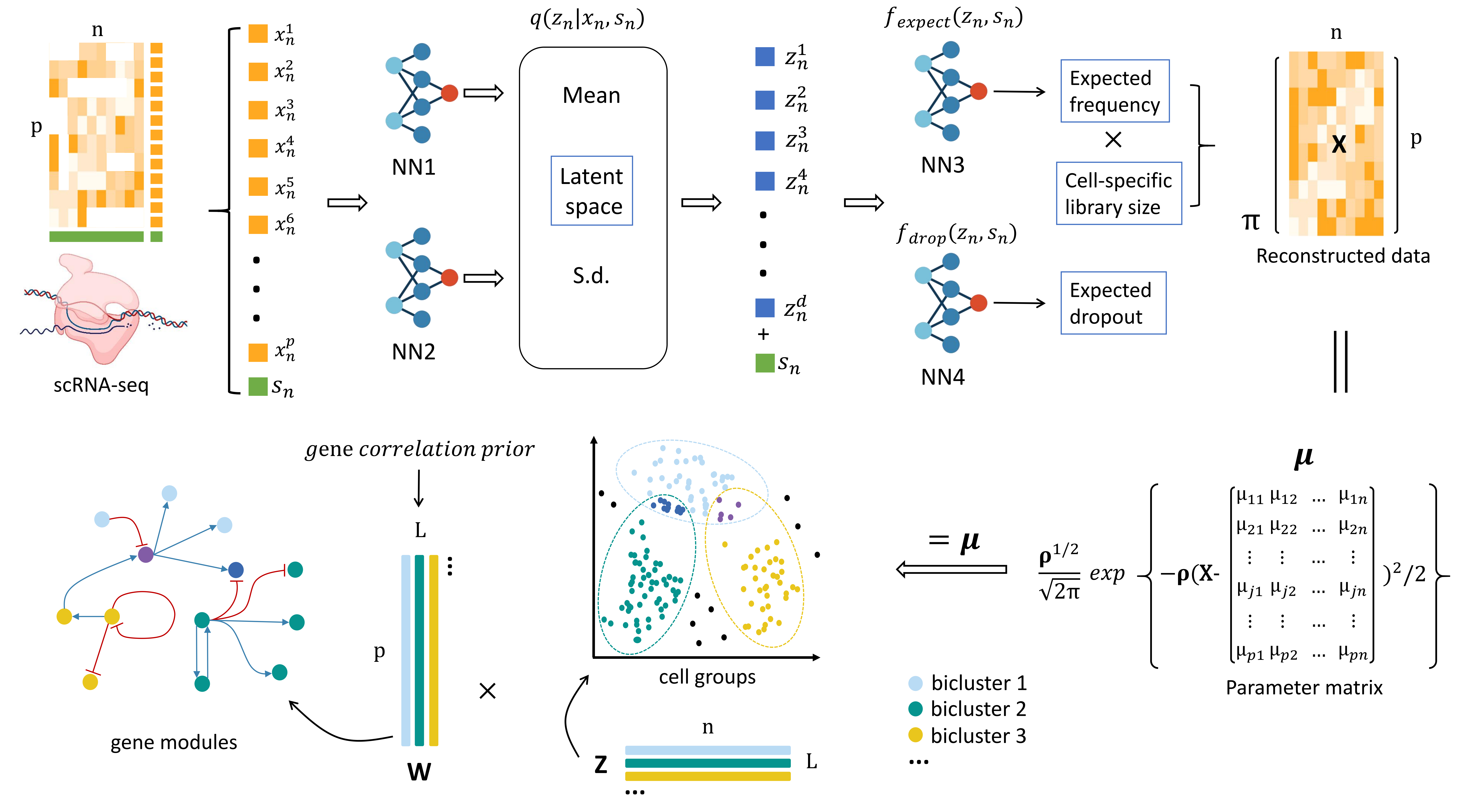
scBC —— a single-cell transcriptome Bayesian biClustering framework.
This document will help you easily go through the scBC model.
Installation
To install our package, run
conda install -c conda-forge scvi-tools #pip install scvi-tools
pip install scBC
Quick start
To simply illustrate how one can run our scBC model, here we use the subsampled HEART dataset as an example. We have prepared four subsampled datasets in advance (HEART, PBMC, LUAD and BC), which can be downloaded locally with simple codes:
from scBC import data
heart = data.load_data("HEART")
If you can't download the data automatically, you can also download them manually from our repository and place them in your working directory.
Now you are ready to set up the scBC model:
from scBC.model import scBC
my_model = scBC(adata=heart,batch_key='cell_source')
Notice that adata must be an AnnData object. batch_key specify the specific column in adata.var to be used as batch annotation.
We first train the VAE model with the default setting:
my_model.train_VI()
Then we can get the reconstructed data, we use 10 posterior samples to estimate the mean expression:
my_model.get_reconst_data(n_samples=10)
Since scBC encourage prior information about genes' co-expression to be provided, before conducting biclustering, we first generate a prior edge. Thankfully, we have also provide an API for automatically generating prior edge from biomart database, just run with default setting:
my_model.get_edge()
Now a edge array has been stored in my_model.edge. Run biclustering will automatically use it, we set the number of biclusters as 3 here:
my_model.Biclustering(L=3)
Take a look at the results:
my_model.S
Or maybe we are more interest in the strong classification result at cell level:
my_model.strong_class()
Parameter lists
Here we give some parameter lists for readers to use flexibly:
model
scBC.model.scBC()
- adata: AnnData object with an observed n $\times$ p matrix, p is the number of measurements and n is the number of subjects.
- layer: if not None, uses this as the key in adata.layers for raw count data.
- batch_key: key in adata.obs for batch information. Categories will automatically be converted into integer categories and saved to adata.obs['_scvi_batch']. If None, assigns the same batch to all the data.
- labels_key: key in adata.obs for label information. Categories will automatically be converted into integer categories and saved to adata.obs['_scvi_labels']. If None, assigns the same label to all the data.
- size_factor_key: key in adata.obs for size factor information. Instead of using library size as a size factor, the provided size factor column will be used as offset in the mean of the likelihood. Assumed to be on linear scale.
- categorical_covariate_keys: keys in adata.obs that correspond to categorical data. These covariates can be added in addition to the batch covariate and are also treated as nuisance factors (i.e., the model tries to minimize their effects on the latent space). Thus, these should not be used for biologically-relevant factors that you do not want to correct for.
- continuous_covariate_keys: keys in adata.obs that correspond to continuous data. These covariates can be added in addition to the batch covariate and are also treated as nuisance factors (i.e., the model tries to minimize their effects on the latent space). Thus, these should not be used for biologically-relevant factors that you do not want to correct for.
Attributes
self.adata- The AnnData used when initializing the scBC object.self.p- Number of measurements(genes) of the expression matrixself.n- Number of subjects(cells) of the expression matrxself.vi_model- The scvi modelself.reconst_data- Reconstructed expression matrix with n $\times$ pself.W- W matrix after biclusteringself.Z- Z matrix after biclusteringself.mu- Parameter matrix $\pmb\mu$ after biclusteringself.convg_trail- The converge trail of biclustering process (likelihood value)self.S- A list containing L dictionaries. The $i_{th}$ dictionary is the $i_{th}$ bicluster's resultsself.niter- Iteration time during biclusteringself.edge- The prior edge array
Methods
scBC.train_VI()
-
n_hidden: Number of nodes per hidden layer.
-
n_latent: Dimensionality of the latent space.
-
n_layers: Number of hidden layers used for encoder and decoder NNs.
-
dropout_rate: Dropout rate for neural networks.
-
dispersion: One of the following:
'gene'- dispersion parameter of NB is constant per gene across cells'gene-batch'- dispersion can differ between different batches'gene-label'- dispersion can differ between different labels'gene-cell'- dispersion can differ for every gene in every cell
-
gene_likelihood: One of:
'nb'- Negative binomial distribution'zinb'- Zero-inflated negative binomial distribution'poisson'- Poisson distribution
-
latent_distribution: One of:
'normal'- Normal distribution'ln'- Logistic normal distribution (Normal(0, I) transformed by softmax)
-
max_epochs: Number of passes through the dataset. If
None, defaults tonp.min([round((20000 / n_cells) * 400), 400]) -
use_gpu: Use default GPU if available (if None or True), or index of GPU to use (if int), or name of GPU (if
str, e.g.,'cuda:0'), or use CPU (if False). -
batch_size: Minibatch size to use during training.
-
early_stopping: Perform early stopping.
scBC.get_reconst_data()
- n_samples: Number of posterior samples to use for estimation.
- batch_size: Minibatch size for data loading into model.
scBC.get_edge()
-
gene_list: A list containing HGNC gene names used to find prior edge in hsapiens_gene_ensembl dataset. Different actions will be performed based on the data type you provide:
str- take self.adata.var[gene_list] as the gene setlist- use the provided list as the gene set to be searchedNone(default)--- use the variable names(self.adata.var_names) as the gene set
-
dataset: The dataset to be used for extracting prior information. Default is hsapiens_gene_ensembl.
-
intensity: A integer denoting the intensity of the prior. Generally speaking, the larger the number, the more prior information returned (the bigger the edge array is).
scBC.Biclustering()
- L: number of the maximum biclusters
- mat: a p x n numpy array used for biclustering. We will use the reconstructed data after calling scBC.get_reconst_data(). However, you can explicitly provide one rather than using the reconstructed data.
- edge: a 2-colounm matrix providing prior network information of some measurements. We prefer to use the edge given here, if not provided, we will use scBC.edge as a candidate. Edge can be automaticly generated using scBC.get_edge(). Running Biclustering() without any edge prior is also feasible.
- dist_type: a p-element vector, each element represents the distribution type of measurements. 0 is Gaussian, 1 is Binomial, 2 is Negative Binomial, 3 is Poisson. If not given, all measurements are deemed to follow Gaussian distribution.
- param: a p-element vector, each element is the required parameter for the correspondence distribution. $\zeta$ for Gaussian, $n_j$ for Binomial, $r_j$ for Negative Binomial, $N$ for Poisson. Default is set as a 1 vector.
- initWZ: select between "random" and "svd". If "random", randomly generated N(0,1) numbers are used, o.w. use SVD results for initialization.
- maxiter: allowed maximum number of iterations.
- tol: desired total difference of solutions.
simulation
We also provide an API for simulation in scBC.data:
scBC.data.simulate_data()
- L: number of biclusters
- p: number of measurements(genes)
- n: number of objects(cells)
- dropout: dropout rate (between 0 and 1)
- batch_num: number of batches you want to simulate
return value
A dictionary containing several simulation results:
| key | word |
|---|---|
| W | The W matrix |
| Z | The Z matrix |
| dat | AnnData object with expression matrix (n $\times$ p) |
| S | The ground truth result |
| edge | Randomly generated prior edge array |
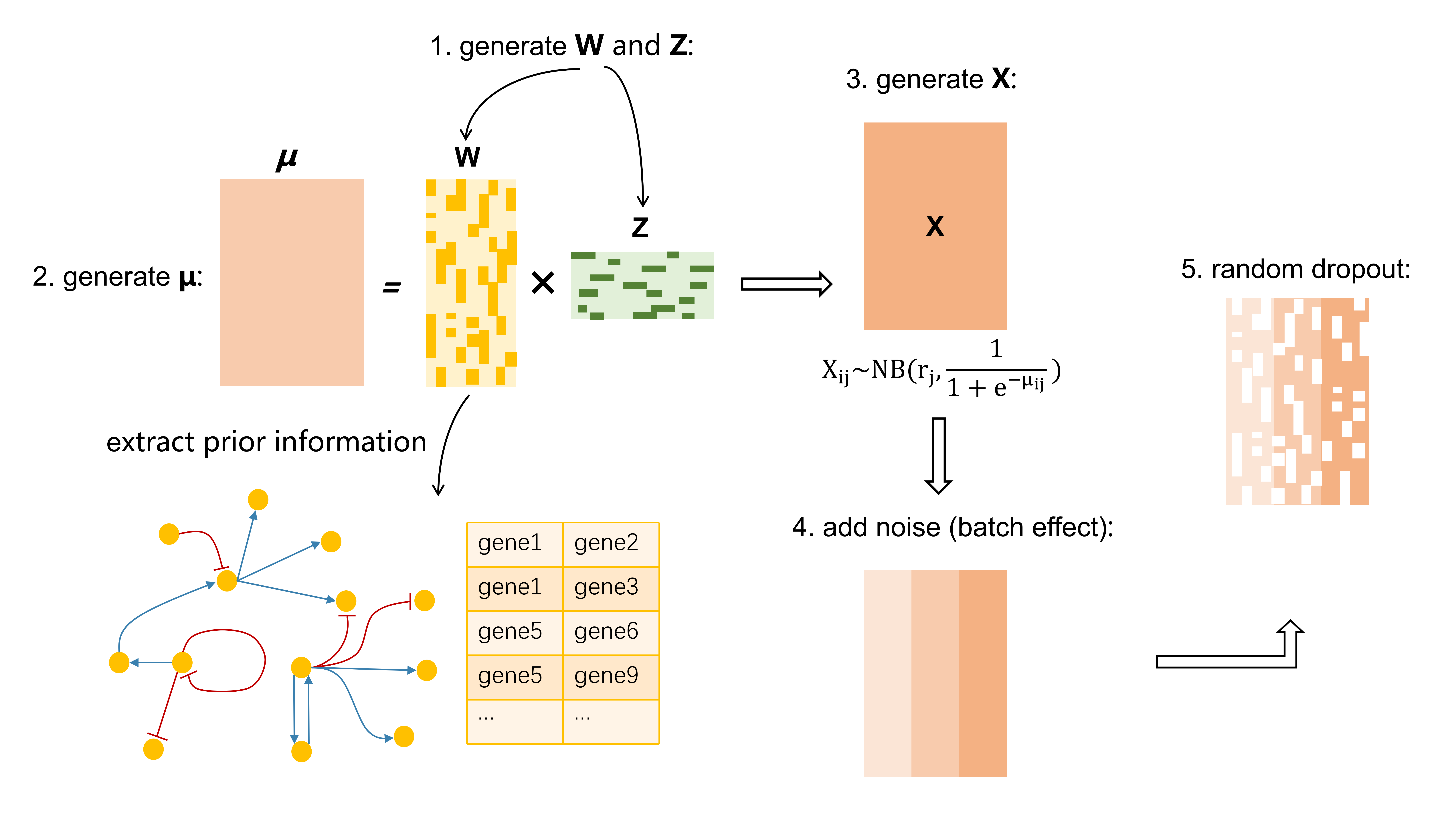
During simulation, the scale of the FGM increases adaptively with the size of the simulated dataset (actually the size of p). The parameter $\pmb\mu$ is computed by the multiplicative model $\pmb\mu = \pmb{WZ}$, where W is a p×L matrix and Z is an L×n matrix. The number of non-zero elements in each column of W is set as p/20, and the number of non-zero elements in each row of Z is set as n/10. The row indices of non-zero elements in W and the column indices of Z with non-zero elements are randomly drawn from 1 to p and 1 to n. The nonzero element values for both W and Z are generated from a normal distribution with mean 1.5 and standard deviation 0.1, and are randomly assigned to be positive or negative. The prior edge is generated along with W. When generating X, each element is generated from $NB(r_j,\frac1{1+e^{-\mu_{ij}}})$ , and the parameter is randomly drawn from 5 to 20. Finally, in order to simulate different batches, we divided the dataset into batch_num parts, each with different intensities of noise. The implementation of dropout is to perform Bernoulli censoring at each data point according to the given dropout rate parameter. The simulation data generation process is shown as follows.
1 maintainer

Metadata
1 maintainer
Release files for scBC 0.3.2
For a detailed explanation of source distributions (sdists) and built distributions (wheels), please see the package formats documentation.
Source distribution (sdist)
| File | Size | Uploaded | Provenance | Actions |
|---|---|---|---|---|
| scBC-0.3.2.tar.gz | 16.8 kB | Without provenance | Details for scBC-0.3.2.tar.gz |
Built distribution (wheel)
| File | Interpreter | ABI | Platform | Actions Reset |
|---|---|---|---|---|
| scBC-0.3.2-py3-none-any.whl | Python 3 | none | any | Details for scBC-0.3.2-py3-none-any.whl |
Total release size: 31.9 kB
Release files / scBC-0.3.2.tar.gz
| Download URL | scBC-0.3.2.tar.gz |
|---|---|
| Size | 16.8 kB |
| Tags | Source |
|
SHA-256 checksum How to use checksums |
bf08ae1089e998f72328e23b53a3a957471a0c24406a764e7433d684e25fce71
|
|
BLAKE2b-256 checksum How to use checksums |
34e275a1d1ddcf2181f854c6ccba2c215fd90bdf728f4fdcb60df134b668188a
|
| Upload date | |
|
Uploaded using Trusted Publishing? What is trusted publishing? |
No |
| Uploaded via |
twine/5.0.0 CPython/3.9.18
|
Release files / scBC-0.3.2-py3-none-any.whl
| Download URL | scBC-0.3.2-py3-none-any.whl |
|---|---|
| Size | 15.1 kB |
| Tags | Python 3 |
|
SHA-256 checksum How to use checksums |
b7fc024ee456e366a82dc62c18a586efe0dbcb0718c678562ba5e74515c4beca
|
|
BLAKE2b-256 checksum How to use checksums |
24a64aa35c9f45741852c0e1179b64aa74d657a42004baa86cce9c859534cd92
|
| Upload date | |
|
Uploaded using Trusted Publishing? What is trusted publishing? |
No |
| Uploaded via |
twine/5.0.0 CPython/3.9.18
|
Security for scBC 0.3.2
Provenance
Provenance describes where a file came from. On PyPI, provenance is shared via attestations, which provide a verifiable record of the build or publishing details. View details, limitations and caveats.
No provenance found
None of the files in this release were uploaded with provenance metadata.
A note on package security
PyPI is a repository for distributing packages, not a service for auditing them. While third-party security researchers and our staff do their best to detect and remove malicious packages, PyPI cannot guarantee the quality, security or suitability of any given package.
To learn more about protecting yourself from malicious actors, visit our package security documentation.














