SLIX allows an automated evaluation of SLI measurements and generates different parameter maps.

Project description


Documentation wiki: https://3d-pli.github.io/SLIX/
SLIX – Scattered Light Imaging ToolboX

- Introduction
- System recommendations
- Installation of SLIX
- Evaluation of SLI Profiles
- Generation of Parameter Maps
- Visualization of Parameter Maps
- Cluster parameters
- Tutorial
- Performance Metrics
- Authors
- References
- Acknowledgements
- License
Introduction
Scattered Light Imaging (SLI) is a novel neuroimaging technique that allows to explore the substructure of nerve fibers, especially in regions with crossing nerve fibers, in whole brain sections with micrometer resolution (Menzel et al. (2020)). By illuminating histological brain sections from different angles and measuring the transmitted light under normal incidence, characteristic light intensity profiles (SLI profiles) can be obtained which provide crucial information such as the directions of crossing nerve fibers in each measured image pixel.
This repository contains the Scattered Light Imaging ToolboX (SLIX) – an open-source Python package that allows a fully automated evaluation of SLI measurements and the generation of different parameter maps. The purpose of SLIX is twofold: First, it allows to transform the raw data of SLI measurements (SLI image stack) to human-readable parameter maps that can be used for further analysis and interpreted by researchers. To this end, SLIX also contains functions to visualize the resulting parameter maps, e.g. as colored vector maps. Second, the results of SLIX can be processed further for use in tractography algorithms. For example, the resulting fiber direction maps can be stored as angles or as unit vectors, which can be used as input for streamline tractography algorithms (Nolden et al. (2019)).
The figure belows shows the different steps, from the SLI measurement to the generation of parameter maps:
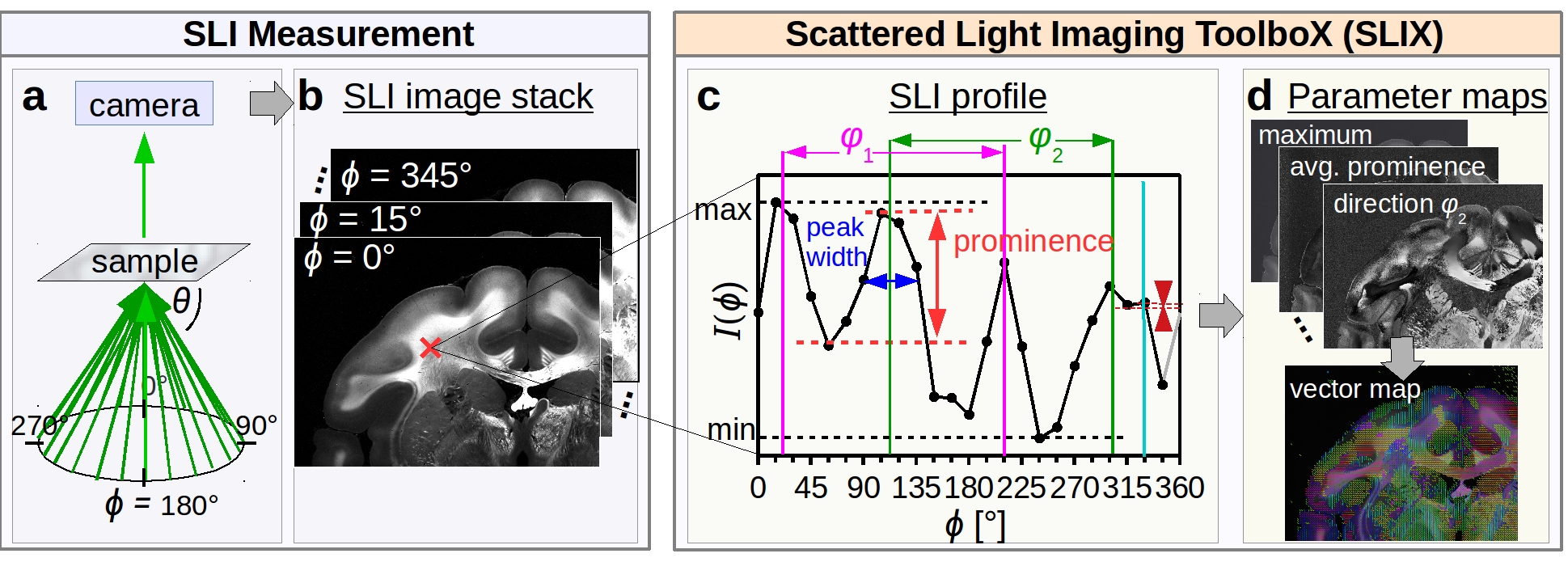
SLI Measurement
The sample is illuminated from different angles, with constant polar angle 

The SLI image stack is used as input for SLIX (.nii or .tiff are accepted). The software assumes that the measurement has been performed with equidistant angles over a full range of 360°. The number of images defines the illumination angles (e.g. when using 24 images as input, the software assumes that the images were recorded with
SLI Profiles
Each pixel in the SLI image stack contains a light intensity profile (SLI profile 
The peak positions are computed with scipy.signal.find_peaks, taking the 360° periodicity of the signal into account. To account for inaccuracies introduced by the discretization of the SLI profile, the determined peak positions are corrected by calculating the geometric center of the peak tips with a height corresponding to 6% of the total signal amplitude. The value of 6% turned out to be the best choice to obtain reliable fiber orientations (see Menzel et al. (2020), Appx. B), but can be changed by the user. Figure (c) shows an SLI profile with 15° discretization and the corrected peak positions as vertical lines.
To avoid that peaks caused by noise or details in the fiber structure impair the computed fiber direction angles, only prominent peaks are used for further evaluation. The peak prominence (scipy.signal.peak_prominences) indicates how strongly a peak stands out from the background signal and is defined by the vertical distance between the top of the peak and the higher of the two neighboring minima (see figure (c), in red). If not defined otherwise by the user, peaks with a prominence above 8% of the total signal amplitude (max-min) are considered as prominent peaks. The value of 8% turned out to be the optimal choice for the generation of reliable fiber orientations (best compromise between correctly and wrongly detected peaks for regions with known fiber orientations, see Menzel et al. (2020), Appx. A).
The peak width (see figure (c), in dark blue) is determined as the full width of the peak at a height corresponding to the peak height minus half of the peak prominence.
The in-plane fiber direction angles 
Parameter Maps
By evaluating the SLI profiles of each image pixel, SLIX generates different parameter maps, which provide various information about the investigated brain tissue:
- The average map shows the overall scattering of the tissue; maximum and minimum can be used to get an idea of the signal amplitude and the signal-to-noise ratio.
- The number of non-prominent peaks and the number of prominent peaks indicate the clarity of the signal (regions with indefinite scattering signals, such as background or regions with a small number of nerve fibers, show a higher number of non-prominent peaks); the average peak prominence indicates the reliability of the peak positions.
- The average peak width and the peak distance correlate with the out-of-plane angle of the nerve fibers (in-plane fibers show two narrow peaks with a large distance of about 180°).
- The direction maps show the in-plane direction angles of the nerve fibers for up to three different crossing fibers. The fiber directions can be represented by a colored vector map, as described in the tutorial below.
With SLIXLineplotParameterGenerator, it is possible to evaluate individual SLI profiles and compute characteristics such as the number of peaks, their positions, and in-plane fiber direction angles. For a given SLI image stack, SLIXParameterGenerator computes the desired parameter maps for all image pixels.
System recommendations
- Operating System: Windows, Linux, MacOS
- Python version: Python 3.6+
- Processor: At least four threads if executed on CPU only
- RAM: 8 GiB or more
- (optional GPU: NVIDIA GPU supported by CUDA 9.0+)
Installation of SLIX
Install SLIX via PyPI
Installing the currently available version of SLIX through PyPI is the recommended way. Use the following command to install SLIX into your Python enviroment.
pip install SLIX
How to install SLIX as Python package from source
If you want to use the latest available version from the GitHub repository, you can use the following commands. Please note that features available here in comparison to the PyPI release might still be in development.
git clone git@github.com:3d-pli/SLIX.git
cd SLIX
pip install .
How to clone SLIX (for further work)
If you want to contribute to SLIX, clone the repository and install the requirements in a virtual environment like seen below.
git clone git@github.com:3d-pli/SLIX.git
cd SLIX

# A virtual environment is recommended:
python3 -m venv venv
source venv/bin/activate

pip install -r requirements.txt
Evaluation of SLI Profiles
SLIXLineplotParameterGenerator allows the evaluation of individual SLI profiles (txt-files with a list of intensity values): For each SLI profile, the maximum, minimum, number of prominent peaks, corrected peak positions, fiber direction angles, and average peak prominence are computed and stored in a text file. The user has the option to generate a plot of the SLI profile that shows the profile together with the peak positions before/after correction. The corrected peak positions are determined by calculating the geometric center of the peak tip, improving the accuracy of the determined peak positions in discretized SLI profiles. If not defined otherwise, the peak tip height corresponds to 6% of the total signal amplitude (for derivation, see Menzel et al. (2020), Appx. B).
SLIXLineplotParameterGenerator -i [INPUT-TXT-FILES] -o [OUTPUT-FOLDER] [[parameters]]
Required Arguments
| Argument | Function |
|---|---|
-i, --input |
Input text files, describing the SLI profiles (list of intensity values). |
-o, --output |
Output folder used to store the characteristics of the SLI profiles in a txt-file (Max, Min, Num_Peaks, Peak_Pos, Directions, Prominence). Will be created if not existing. |
Optional Arguments
| Argument | Function |
|---|---|
--smoothing [args] |
Apply smoothing to the SLI profiles for each image pixel before evaluation. Available options are low pass fourier filtering fourier and Savitzky-Golay filtering savgol. With both options, you can input up to two numbers to specify the parameters for the smoothing algorithm. With fourier, you are able to choose soft threshold for the fourier filter in percent 0.2 = 20% and a smoothing multiplier (range 0--1, higher values mean more smoothing) (e.g. fourier 0.1 0.02). With Savitzky-Golay you can choose the window length and the polynomial order (e.g. savgol 45 2) |
--prominence_threshold |
Change the threshold for prominent peaks. Peaks with lower prominences will not be used for further evaluation. (Default: 8% of total signal amplitude.) Only recommended for experienced users! (default: 0.08) |
--without_angles |
Scatterometry measurements typically include the measurment angle in their text files. Enable this option if you have line profiles which do not have angles for each measurement. Keep in mind, that the angles will be ignored regardless. SLIX will generate the parameters based on the number of measurement angles. |
--simple |
Replace most output parameters by a single value which represents the mean value of the given parameter in the line profile. |
Example
The following example demonstrates the evaluation of two SLI profiles, which can be found in the "examples" folder of the SLIX repository:
SLIXLineplotParameterGenerator -i examples/*.txt -o output --without_angles
The resulting plot and txt-file are shown below, exemplary for one of the SLI profiles (90-Stack-1647-1234.txt):
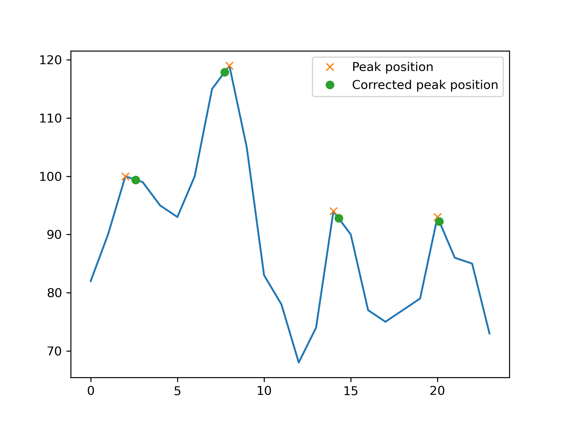
profile,82.0,90.0,100.0,99.0,95.0,93.0,100.0,115.0,119.0,105.0,83.0,78.0,68.0,74.0,94.0,90.0,77.0,75.0,77.0,79.0,93.0,86.0,85.0,73.0
filtered,82.0,90.0,100.0,99.0,95.0,93.0,100.0,115.0,119.0,105.0,83.0,78.0,68.0,74.0,94.0,90.0,77.0,75.0,77.0,79.0,93.0,86.0,85.0,73.0
centroids,0.0,0.0,0.5981955528259277,0.0,0.0,0.0,0.0,0.0,-0.27211764454841614,0.0,0.0,0.0,0.0,0.0,0.2986946105957031,0.0,0.0,0.0,0.0,0.0,0.10755850374698639,0.0,0.0,0.0
peaks,False,False,True,False,False,False,False,False,True,False,False,False,False,False,True,False,False,False,False,False,True,False,False,False
significant peaks,False,False,True,False,False,False,False,False,True,False,False,False,False,False,True,False,False,False,False,False,True,False,False,False
prominence,0.0,0.0,0.07887327671051025,0.0,0.0,0.0,0.0,0.0,0.5746479034423828,0.0,0.0,0.0,0.0,0.0,0.236619770526886,0.0,0.0,0.0,0.0,0.0,0.202816903591156,0.0,0.0,0.0
width,0.0,0.0,29.625,0.0,0.0,0.0,0.0,0.0,66.76947784423828,0.0,0.0,0.0,0.0,0.0,30.375001907348633,0.0,0.0,0.0,0.0,0.0,40.89285659790039,0.0,0.0,0.0
distance,0.0,0.0,175.5074920654297,0.0,0.0,0.0,0.0,0.0,185.6951446533203,0.0,0.0,0.0,0.0,0.0,184.4925079345703,0.0,0.0,0.0,0.0,0.0,174.3048553466797,0.0,0.0,0.0
direction,143.27333068847656,61.23419189453125,-1.0
The plot shows the SLI profile derived from a stack of 24 images. The x-axis displays the number of images, the y-axis the measured light intensity [a.u.]. To detect peaks at the outer boundaries, SLIX uses a derived version of SciPys peak finding algorithm which is extended to respect boundary regions; The dots are the original peak positions. The crosses indicate the corrected peak positions, taking the discretization of the profile into account.
The resulting .csv file will contain detailed information of each feature SLIX can compute. Here, the filtered profile, as well as the peaks, significant peaks, centroids and more will be shown in a per-measurement basis. This allows a detailed analysis of the data.
When adding the --simple option, the output will be much simpler reducing most parameters to a single value instead.
Running the following code example:
SLIXLineplotParameterGenerator -i examples/*.txt -o output --without_angles --simple
will yield the following .csv file instead
profile,82.0,90.0,100.0,99.0,95.0,93.0,100.0,115.0,119.0,105.0,83.0,78.0,68.0,74.0,94.0,90.0,77.0,75.0,77.0,79.0,93.0,86.0,85.0,73.0
filtered,82.0,90.0,100.0,99.0,95.0,93.0,100.0,115.0,119.0,105.0,83.0,78.0,68.0,74.0,94.0,90.0,77.0,75.0,77.0,79.0,93.0,86.0,85.0,73.0
centroids,0.0,0.0,0.5981955528259277,0.0,0.0,0.0,0.0,0.0,-0.27211764454841614,0.0,0.0,0.0,0.0,0.0,0.2986946105957031,0.0,0.0,0.0,0.0,0.0,0.10755850374698639,0.0,0.0,0.0
peaks,4
significant peaks,4
prominence,0.27323946356773376
width,41.915584564208984
distance,174.9061737060547
direction,143.27333068847656,61.23419189453125,-1.0
Generation of Parameter Maps
SLIXParameterGenerator allows the generation of different parameter maps from an SLI image stack.
SLIXParameterGenerator -i [INPUT-STACK] -o [OUTPUT-FOLDER] [[parameters]]
Required Arguments
| Argument | Function |
|---|---|
-i, --input |
Input file: SLI image stack (as .tif(f) or .nii). |
-o, --output |
Output folder where resulting parameter maps (.tiff) will be stored. Will be created if not existing. |
Optional Arguments
| Argument | Function |
|---|---|
--thinout |
Average every NxN pixels in the SLI image stack and run the evaluation on the resulting (downsampled) images. (Default: N=1) |
--with_mask |
Consider all image pixels with low scattering as background: Pixels for which the maximum intensity value of the SLI profile is below a defined threshold (--mask_threshold) are set to zero and will not be further evaluated. |
--correctdir |
Correct the resulting direction angle by a floating point value (in degree). This is useful when the stack or camera was rotated. |
--smoothing [args] |
Apply smoothing to the SLI profiles for each image pixel before evaluation. Available options are low pass fourier filtering fourier and Savitzky-Golay filtering savgol. With both options, you can input up to two numbers to specify the parameters for the smoothing algorithm. With fourier, you are able to choose soft threshold for the fourier filter in percent 0.2 = 20% and a smoothing multiplier (range 0--1, higher values mean more smoothing) (e.g. fourier 0.1 0.02). With Savitzky-Golay you can choose the window length and the polynomial order (e.g. savgol 45 2) |
--prominence_threshold |
Change the threshold for prominent peaks. Peaks with lower prominences will not be used for further evaluation. (Default: 8% of total signal amplitude.) Only recommended for experienced users! |
--detailed |
Save 3D images in addition to 2D mean images which include more detailed information but will need a lot more disk space. |
--disable_gpu |
Use the CPU in combination with Numba instead of the GPU variant. This is only recommended if your GPU is significantly slower than your CPU. |
--no_centroids |
Disable centroid calculation for the parameter maps. This is absolutely not recommended and will result in worse parameter maps but can lower the computing time significantly. |
--output_type |
Define the output data type of the parameter images. Default = tiff. Supported types: nii, h5, tiff. (default: tiff) |
The arguments listed below determine which parameter maps will be generated from the SLI image stack. If any such argument (except –-optional) is used, no parameter map besides the ones specified will be generated. If none of these arguments is used, all parameter maps except the optional ones will be generated: peakprominence, number of (prominent) peaks, peakwidth, peakdistance, direction angles in crossing regions.
| Argument | Function |
|---|---|
--peakprominence |
Generate a parameter map (_peakprominence.tiff) containing the average prominence (scipy.signal.peak_prominence) of an SLI profile (image pixel), normalized by the average of the SLI profile. |
--peaks |
Generate two parameter maps (_low_prominence_peaks.tiff and _high_prominence_peaks.tiff) containing the number of peaks in an SLI profile (image pixel) with a prominence below and above the defined prominence_threshold (Default: 8% of the total signal amplitude). |
--peakwidth |
Generate a parameter map (_peakwidth.tiff) containing the average peak width (in degrees) of all prominent peaks in an SLI profile. |
--peakdistance |
Generate a parameter map (_peakdistance.tiff) containing the distance between two prominent peaks (in degrees) in an SLI profile. Pixels for which the SLI profile shows more/less than two prominent peaks are set to -1. |
--direction |
Generate three parameter maps (_dir_1.tiff, _dir_2.tiff, _dir_3.tiff) indicating up to three in-plane direction angles of (crossing) fibers (in degrees). If any or all direction angles cannot be determined for an image pixel, this pixel is set to -1 in the respective map. |
--unit_vectors |
Generate unit vectors maps (.nii) from direction images. |
--inclination_sign |
Generate a direction map not corrected by the 270° and without the restriction to the area of [0°;180°] which allows to search the inclination direction. |
--optional |
Generate four additional parameter maps: average value of each SLI profile (_avg.tiff), maximum value of each SLI profile (_max.tiff), minimum value of each SLI profile (_min.tiff), and in-plane direction angles (in degrees) in regions without crossings (_dir.tiff). Image pixels for which the SLI profile shows more than two prominent peaks are set to -1 in the direction map. |
Example
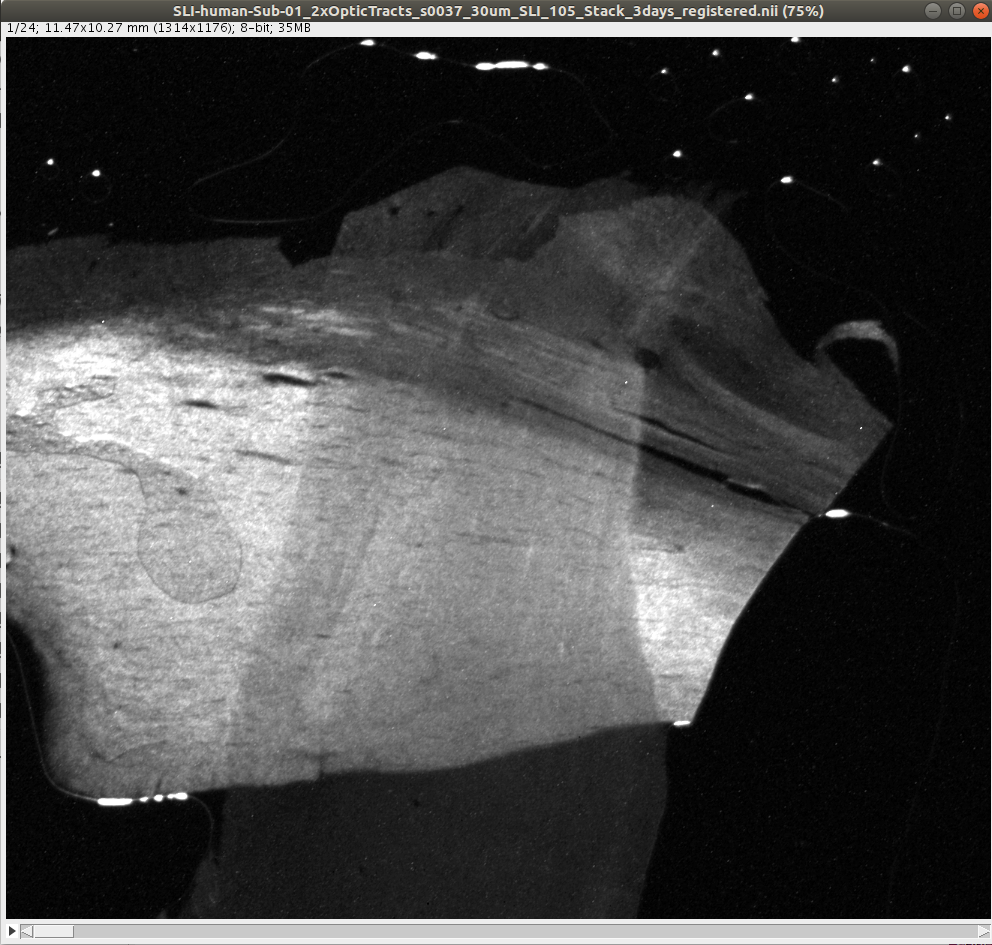
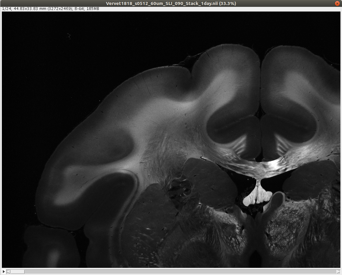
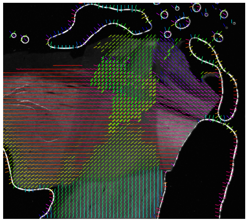
The following example demonstrates the generation of the parameter maps, for two artificially crossing sections of human optic tracts (left) and the upper left corner of a coronal vervet brain section (right):
How to run the demo yourself:
1. Download the needed files:
Command line:
wget https://object.cscs.ch/v1/AUTH_227176556f3c4bb38df9feea4b91200c/hbp-d000048_ScatteredLightImaging_pub/Human_Brain/optic_tracts_crossing_sections/SLI-human-Sub-01_2xOpticTracts_s0037_30um_SLI_105_Stack_3days_registered.nii
wget https://object.cscs.ch/v1/AUTH_227176556f3c4bb38df9feea4b91200c/hbp-d000048_ScatteredLightImaging_pub/Vervet_Brain/coronal_sections/Vervet1818_s0512_60um_SLI_090_Stack_1day.nii
Links:
SLI-human-Sub-01_2xOpticTracts_s0037_30um_SLI_105_Stack_3days_registered.nii
Vervet1818_s0512_60um_SLI_090_Stack_1day.nii
2. Run SLIX:
SLIXParameterGenerator -i ./SLI-human-Sub-01_2xOpticTracts_s0037_30um_SLI_105_Stack_3days_registered.nii -o . --thinout 5

SLIXParameterGenerator -i ./Vervet1818_s0512_60um_SLI_090_Stack_1day.nii -o . --thinout 10 --direction
The execution of both commands should take around one minute max. The resulting parameter maps will be downsampled. To obtain full resolution parameter maps, do not use the roisize option. In this case, the computing time will be higher (around 25 times higher for the first example and 100 times higher for the second example).
To display the resulting parameter maps, you can use e.g. ImageJ or Fiji. More examples (SLI image stacks and resulting parameter maps) can be found on the EBRAINS data repository.
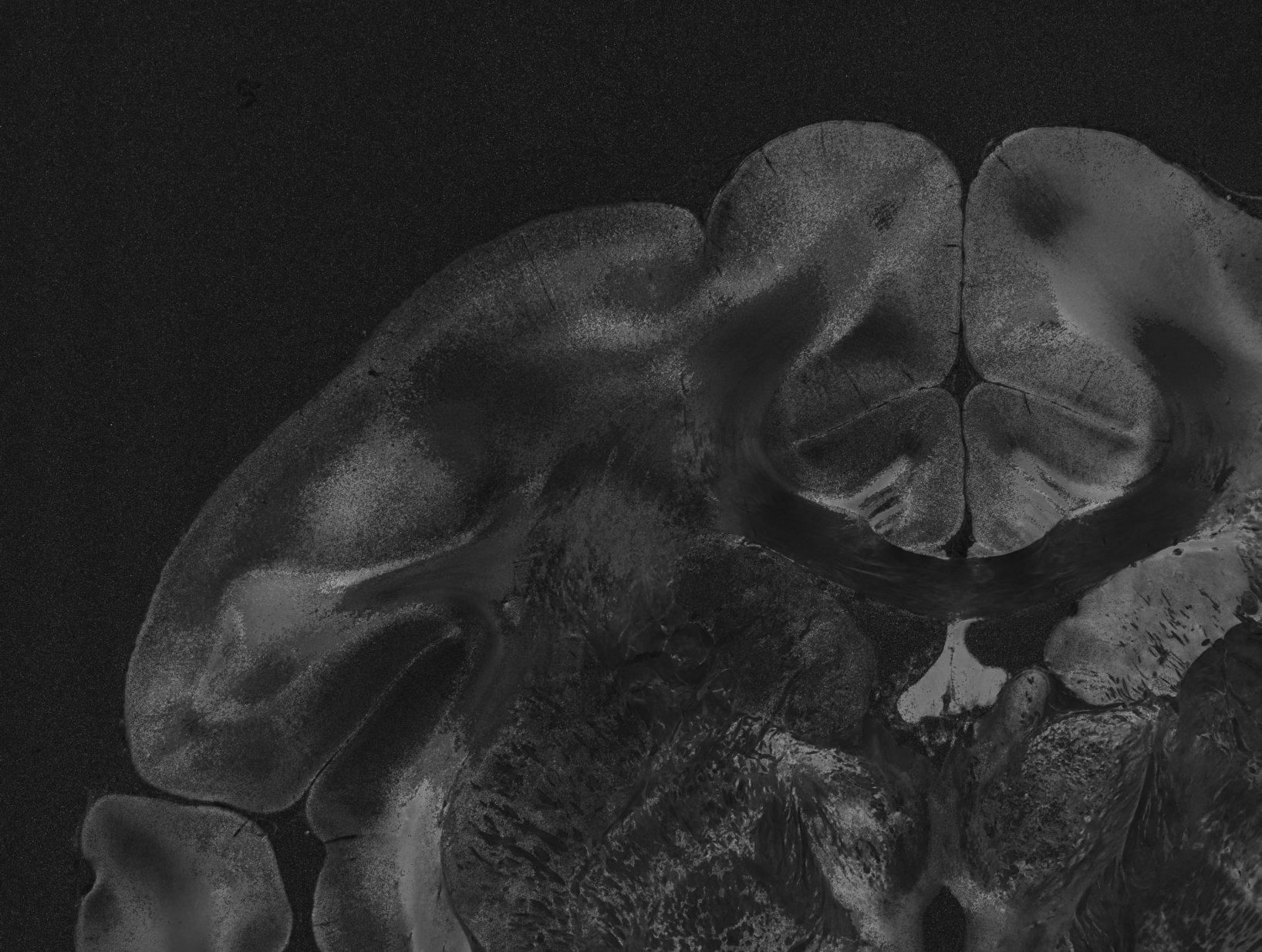
Resulting Parameter Maps
All 12 parameter maps that can be generated with SLIX are shown below, exemplary for the coronal vervet brain section used in the above demo (available here). In contrast to the above demo, the parameter maps were generated with full resolution. For testing purposes, we suggest to run the evaluation on downsampled images, e.g. with --thinout 3, which greatly speeds up the generation of the parameter maps.
SLIXParameterGenerator -i ./Vervet1818_s0512_60um_SLI_090_Stack_1day.nii -o .
Average
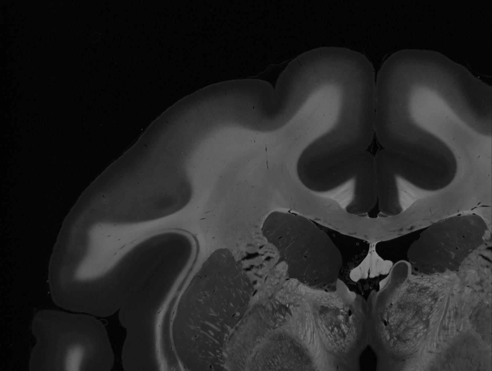
_average.tiff shows the average intensity for each SLI profile (image pixel). Regions with high scattering show higher values.
Low Prominence Peaks
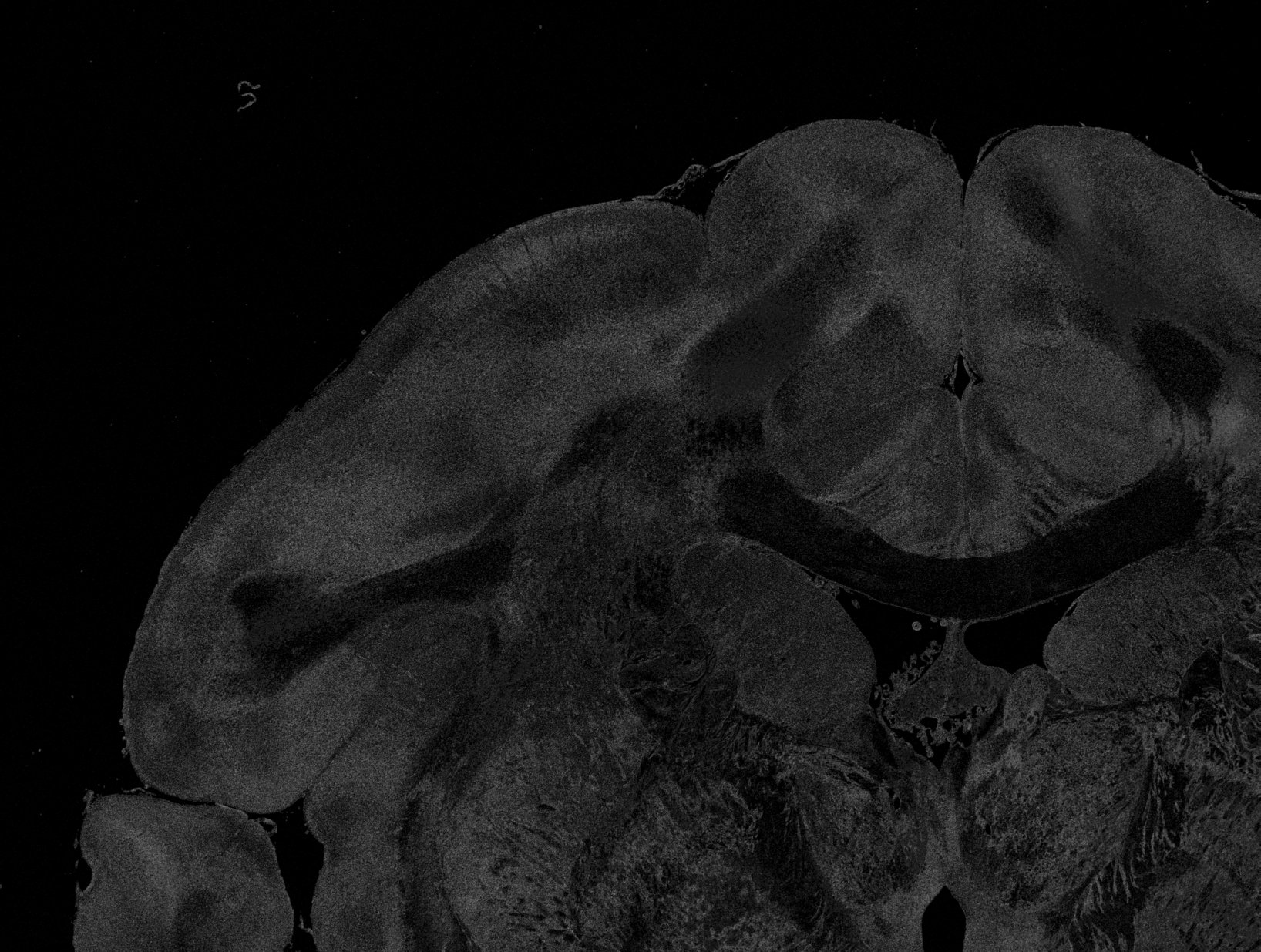
_low_prominence_peaks.tiff shows the number of non-prominent peaks for each image pixel, i.e. peaks that have a prominence below 8% of the total signal amplitude (max-min) of the SLI profile and are not used for further evaluation. For a reliable reconstruction of the direction angles, this number should be small, ideally zero.
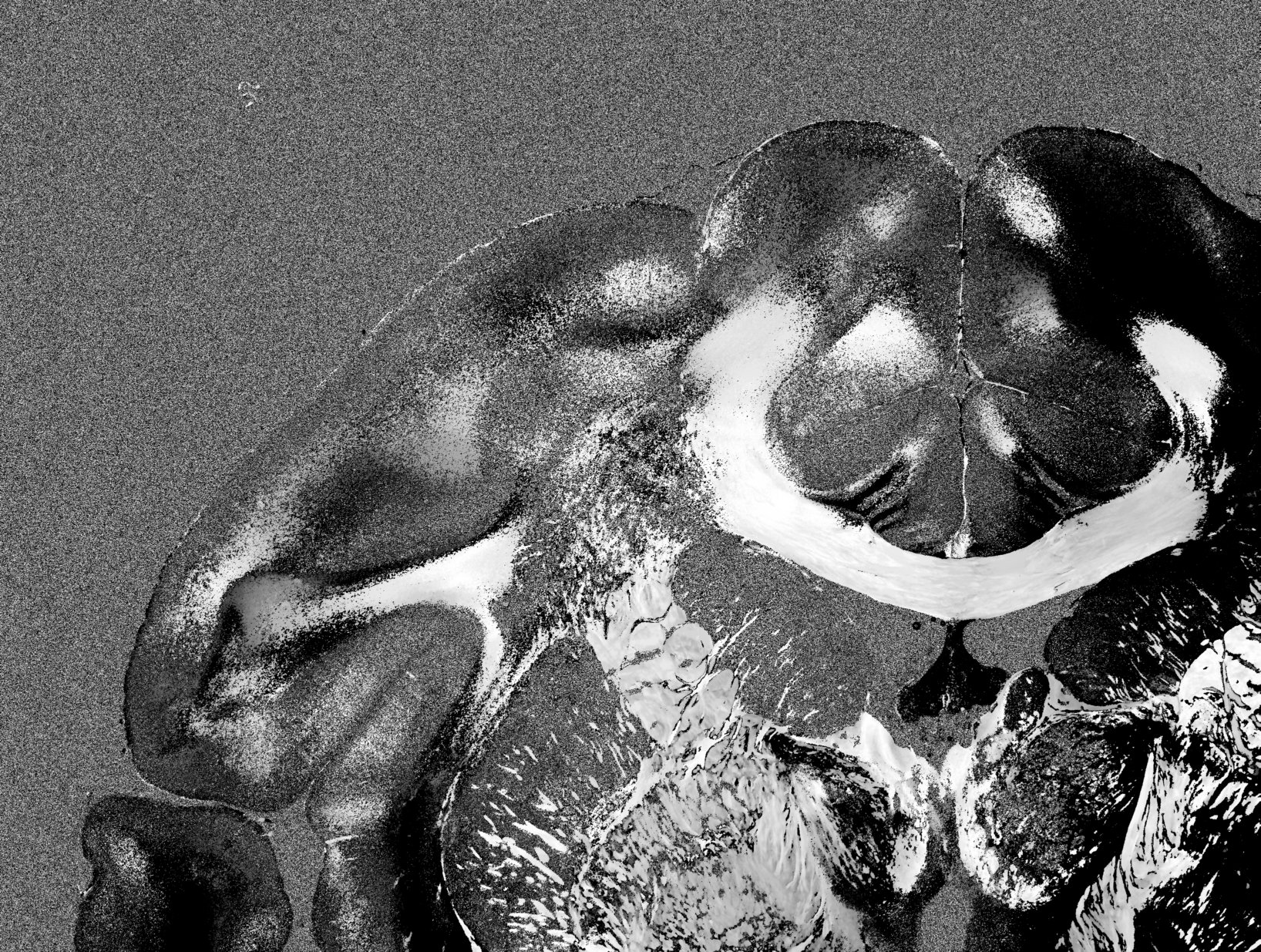
High Prominence Peaks
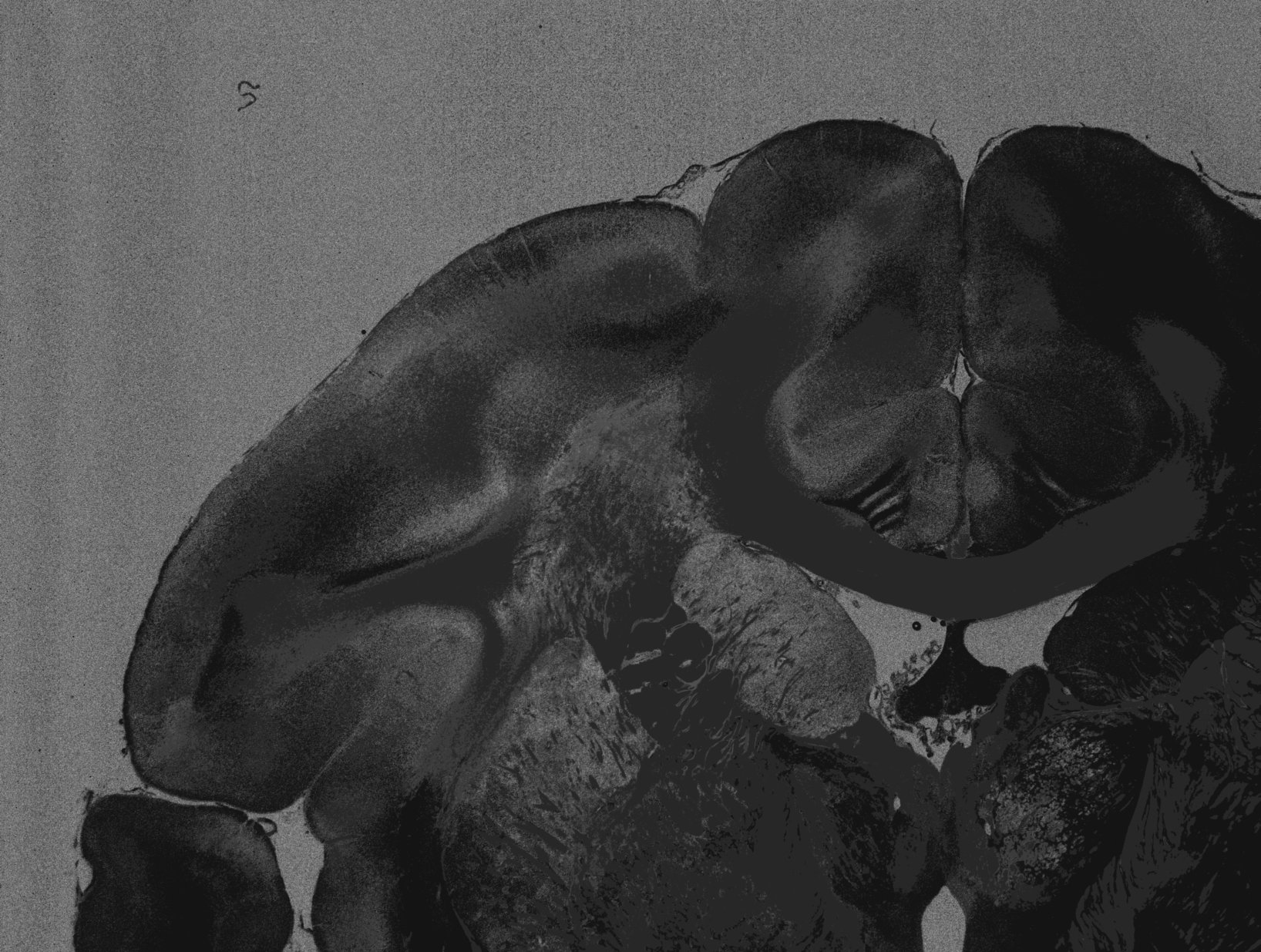
_high_prominence_peaks.tiff shows the number of prominent peaks for each image pixel, i.e. peaks with a prominence above 8% of the total signal amplitude (max-min) of the SLI profile. The position of these peaks is used to compute the fiber direction angles.
Average Peak Prominence
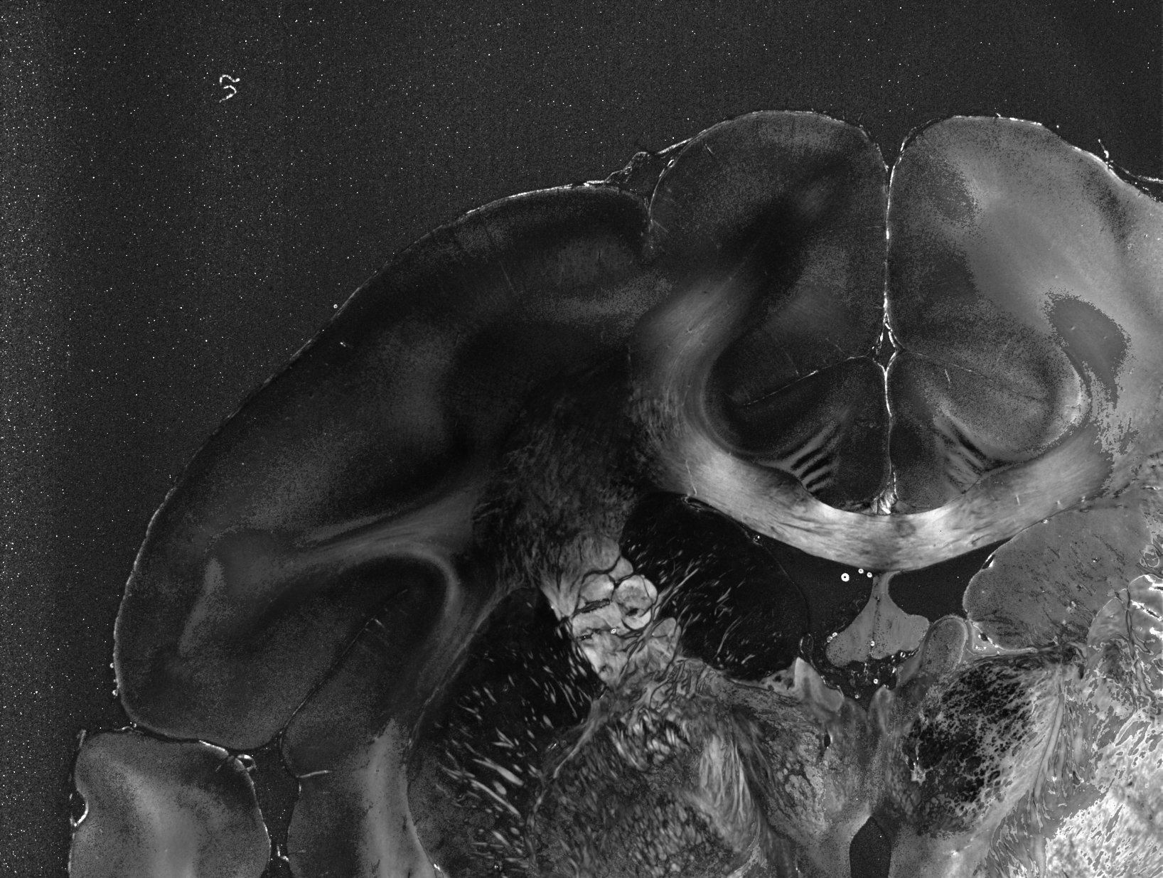
_peakprominence.tiff shows the average prominence of the peaks for each image pixel, normalized by the average of each profile. The higher the value, the clearer the signal.
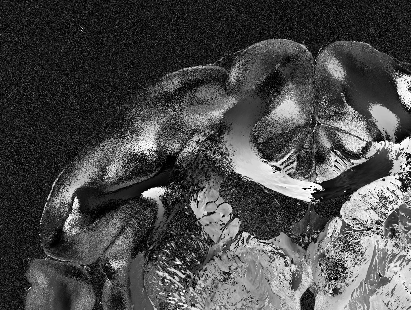
Average Peak Width
_peakwidth.tiff shows the average width of all prominent peaks for each image pixel. A small peak width implies that the fiber directions can be precisely determined. Larger peak widths occur for out-of-plane fibers and/or fibers with small crossing angles.
Peak Distance
_peakdistance.tiff shows the distance between two prominent peaks for each image pixel. If an SLI profile contains only one peak, the distance is zero. In regions with crossing nerve fibers, the distance is not defined and the image pixels are set to -1. The peak distance is a measure for the out-of-plane angle of the fibers: A peak distance of about 180° implies that the region contains in-plane fibers; the more the fibers point out of the section plane, the smaller the peak distance becomes. For fibers with an inclination angle of about 70° and above, a single broad peak is expected.
Direction Angles
The in-plane direction angles are only computed if the SLI profile has one, two, four, or six prominent peaks with a pair-wise distance of (180 +/- 35)°. Otherwise, the image pixel is set to -1. The direction angle is computed from the mid position of one peak pair, or (in case of only one peak) from the position of the peak itself. All direction angles are in degrees (with 0° being along the positive x axis, and 90° along the positive y-axis).
In case of three or five prominent peaks, the peak pairs cannot be safely assigned and are therefore not evaluated. SLI profiles with three peaks could also be caused e.g. by strongly inclined crossing fibers, where a reliable determination of the in-plane fiber directions is not possible. If an SLI profile contains three prominent peaks, it might also be the case that the forth peak lies below the prominence threshold because the signal is not very clear. To account for missing peaks, the user has the possibility to decrease the prominence threshold by setting another value with --prominence_threshold. However, this should be done with caution, as this also causes non-significant peaks that are generated by noise or other artifacts to be considered for evaluation and might yield wrong fiber direction angles. Therefore, we strongly recommend to read the derivation in Menzel et al. (2020), Appx. A, before adjusting the threshold.
_dir_1.tiff shows the first detected fiber direction angle.
_dir_2.tiff shows the second detected fiber direction angle (only defined in regions with two or three crossing fibers).
_dir_3.tiff shows the third detected fiber direction angle (only defined in regions with three crossing fibers).
_dir.tiff shows the fiber direction angle only in regions with one or two prominent peaks, i.e. excluding regions with crossing fibers.
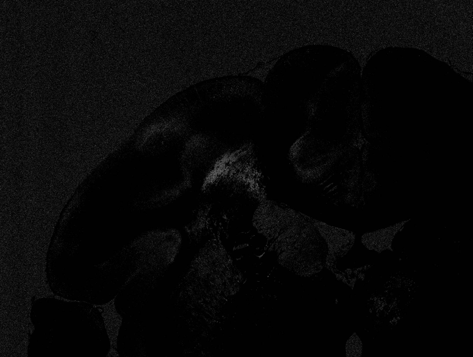
Maximum
_max.tiff shows the maximum of the SLI profile for each image pixel.
Minimum
_min.tiff shows the minimum of the SLI profile for each image pixel.
To obtain a measure for the signal-to-noise, the difference between maximum and minimum can be divided by the average.
Visualization of parameter maps
With SLIXVisualizeParameter the direction can be visualized easily. Just put the direction files as an input argument and generate either fiber orientation maps
or a visualization of the unit vectors easily.
SLIXVisualizeParameter -i [INPUT-DIRECTIONS] -o [OUTPUT-FOLDER] {fom, vector}
Required Arguments
| Argument | Function |
|---|---|
-i, --input, --direction |
Input file: SLI direction stack (as .tif(f) or .nii). |
-o, --output |
Output folder where resulting parameter maps (.tiff) will be stored. |
Optional Arguments
| Argument | Function |
|---|---|
--inclination |
Input file: Inclination (for example registered from 3D-PLI). The inclination file will only influence the color of the shown vectors / FOM and does not change the shown vector orientation itself. |
-c, --colormap |
Changes the color map used for the visualization. Available options: rgb, hsvBlack, hsvWhite, rgb_r (reverse), hsvBlack_r, hsvWhite_r |
Subarguments
SLIXVisualizeParameter supports both the creation of FOMs of direction images, and the visualization
of unit vectors. Depending on what you want to do, there is an argument which follows the input and output options.
The arguments are either fom for the creation of a FOM, or vector for the creation of a vector visualization
Argument fom
| Argument | Function |
|---|---|
--output_type |
Define the output data type of the parameter images. Default = tiff. Supported types: h5, tiff. |
--value |
Set another mask image which will be used to weight the image through the HSV value operator. The image will be normalized 0-1. If this option isn't used, the value will be one. |
--saturation |
Set another mask image which will be used to weight the image through the HSV saturation operator. The image will be normalized to 0-1. If this option isn't used, the value will be one. |
Argument vector
| Argument | Function |
|---|---|
--slimeasurement |
SLI measurement used for the generation of the direction. Required. |
--alpha |
Factor for the vectors which will be used during visualization. A higher value means that the vectors will be more visible. (Value range: 0 -- 1) |
--thinout |
Thin out vectors by an integer value. A thinout of 20 means that both the x-axis and y-axis are thinned by a value of 20. Default = 20 |
--scale |
Increases the scale of the vectors. A higher scale means that the vectors in the resulting image are longer. This can be helpful if many pixels of the input image are empty but you don't want to use the thinout option to see results. If the scale option isn't used, the vectors are scaled by the thinout option. |
--vector_width |
Change the default vector width shown in the resulting image. This can be useful if only a small number of vectors will be shown (for example when using a large thinout) |
--threshold |
When using the thinout option, you might not want to get a vector for a lonely vector in the base image. This parameter defines a threshold for the allowed percentage of background pixels to be present. If more pixels than the threshold are background pixels, no vector will be shown. (Value range: 0 -- 1) |
--dpi |
Set the image DPI value for Matplotlib. Smaller values will result in a lower resolution image which will be written faster. Larger values will need more computation time but will result in clearer images. Default = 1000dpi |
--distribution |
Instead of using each n-th vector for the visualization (determined by the median vector), instead show all vectors on top of each other. Note: Low alpha values (around 1/alpha) are recommended. The threshold parameter won't do anything when using this parameter |
--weight_map |
Weight the length of all vectors by the given weight map (normalized to the range 0 -- 1) |
Example
# Download the image
wget https://object.cscs.ch/v1/AUTH_227176556f3c4bb38df9feea4b91200c/hbp-d000048_ScatteredLightImaging_pub/Vervet_Brain/coronal_sections/Vervet1818_s0512_60um_SLI_090_Stack_1day.nii

# Generate direction
SLIXParameterGenerator -i Vervet1818_s0512_60um_SLI_090_Stack_1day.nii -o Output/ --direction --with_mask

# Use direction to create a FOM
SLIXVisualizeParameter -i Output/Vervet1818_s0512_60um_SLI_090_Stack_1day_dir_1.tiff Output/Vervet1818_s0512_60um_SLI_090_Stack_1day_dir_2.tiff Output/Vervet1818_s0512_60um_SLI_090_Stack_1day_dir_3.tiff -o Output fom

# Visualize the unit vectors from the direction
SLIXVisualizeParameter -i Output/Vervet1818_s0512_60um_SLI_090_Stack_1day_dir_1.tiff Output/Vervet1818_s0512_60um_SLI_090_Stack_1day_dir_2.tiff Output/Vervet1818_s0512_60um_SLI_090_Stack_1day_dir_3.tiff -o Output vector --slimeasurement Vervet1818_s0512_60um_SLI_090_Stack_1day.nii

# Visualize the unit vector distribution from the direction
SLIXVisualizeParameter -i Output/Vervet1818_s0512_60um_SLI_090_Stack_1day_dir_1.tiff Output/Vervet1818_s0512_60um_SLI_090_Stack_1day_dir_2.tiff Output/Vervet1818_s0512_60um_SLI_090_Stack_1day_dir_3.tiff -o Output vector --slimeasurement Vervet1818_s0512_60um_SLI_090_Stack_1day.nii --distribution --alpha 0.03 --thinout 40 --vector_width 1
Resulting images
FOM
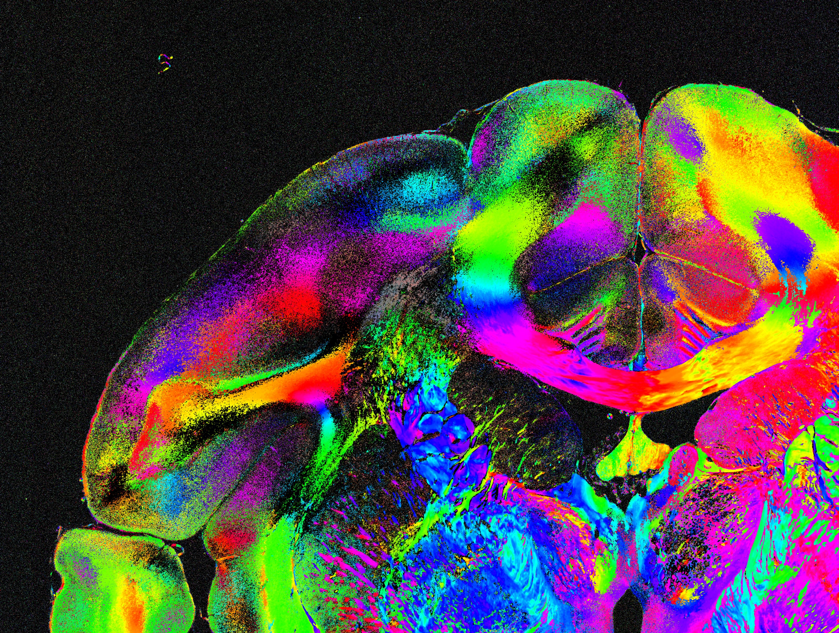
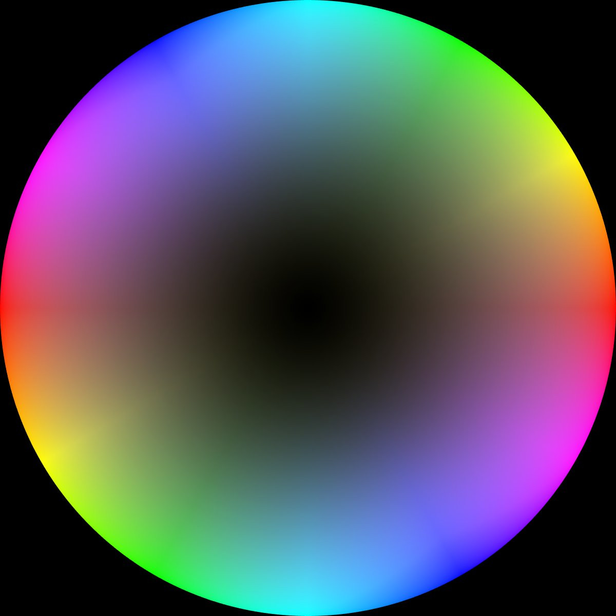
The following color bubble is used for the visualization of the orientation map. The color will match the angle of the direction.
The fiber orientation map, which is generated by SLIXVisualizeParameter presents each pixel of the raw measurement as a four pixel region.
Each pixel in that region will get a color based on the number of directions in the measurement as well as the orientation of each direction.
When only one direction is present, all four pixels will be mapped to the HSV color of that direction.
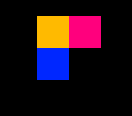
Two directions will be shown in a cross pattern. An example is shown below.
When three directions are present, the first three pixel will have the HSV color of the direction. The fourth pixel will be black (no direction).
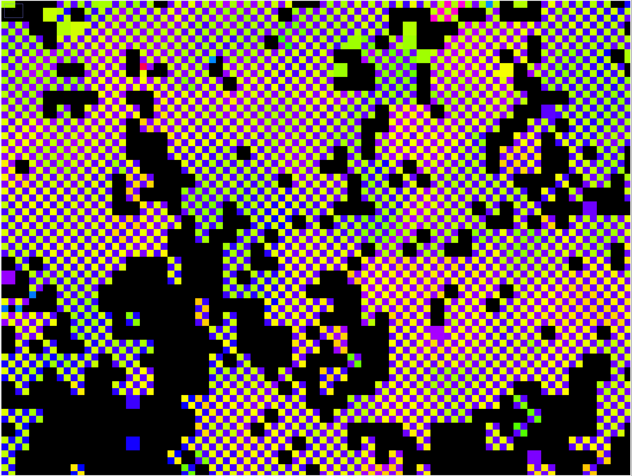
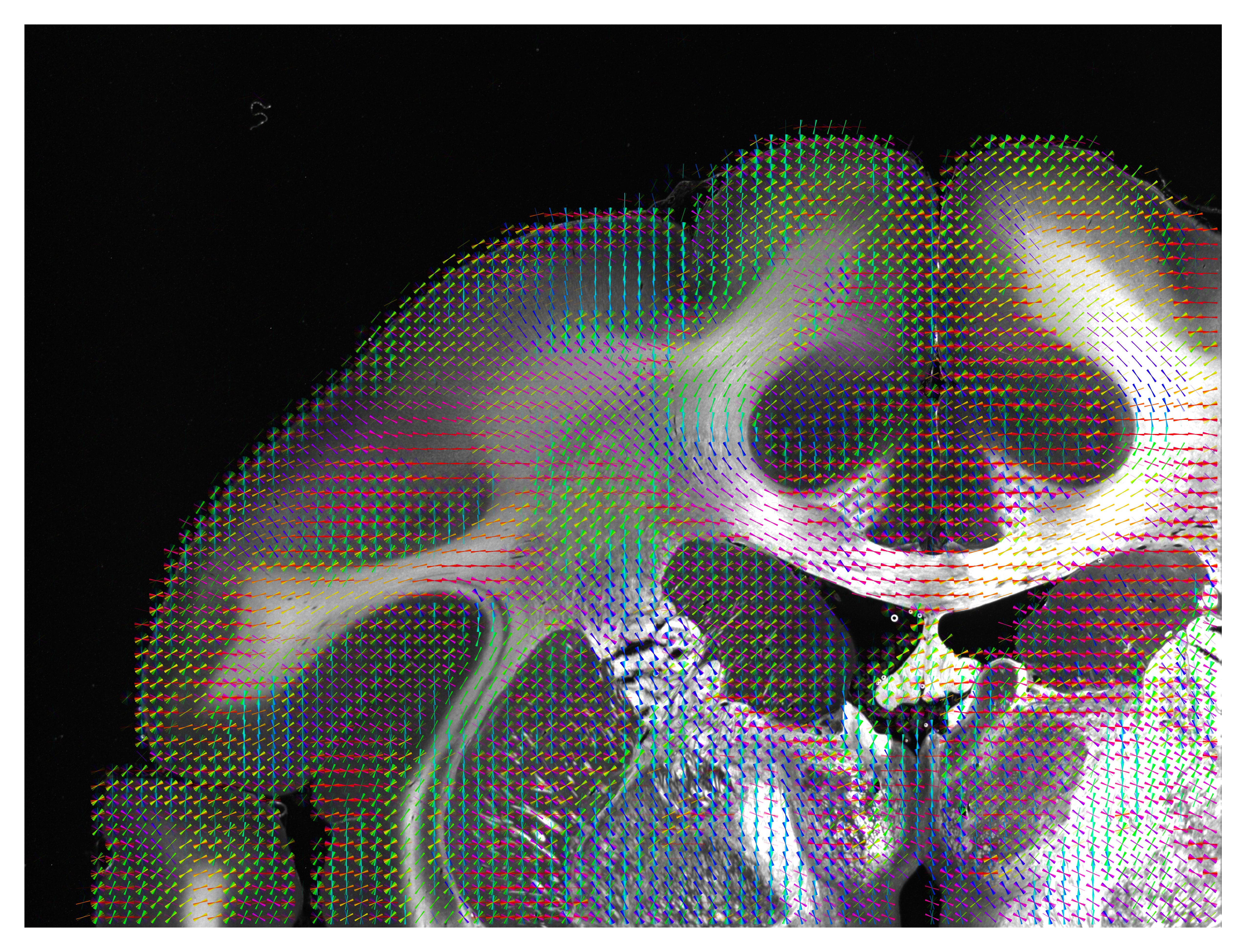
Unit vector map
The unit vector map will contain a selection of unit vectors. The color of the vector will be the angle of the direction. The number of vectors is determined by the thinout parameter. Using the scale option, one can choose to scale the length of the vectors. This option is recommended to get a quick overview of a measurement as the computing time is short in comparison to the FOM or vector distribution. However, not all information about a measurement might be included.
Vector distribution
The vector distribution will always show all unit vectors of a measurement. To archive this while keeping an image which is easy to interpret, multiple vectors will be put on top of each other. This can lead to confusion if one vector appears only once but is still shown with full brightness. Therefore, a low alpha value is absolutely recommended with this option. This visualization method is quite computationally expensive. The color of the vector will be the angle of the direction.
Cluster parameters
With the last tool SLIXCluster, using the parameters of the previous tools, you can generate a cluster map separating flat, crossing and inclinated fibers.
This can help to identify regions which would not be as easy to identify when only looking at a single parameter map.
SLIXCluster uses threshold parameters to separate regions based on findings in recent studies. The resulting parameter map will always be saved as an 8-bit image.
Required parameters
| Argument | Function |
|---|---|
-i, --input |
Input folder with all (including optional) parameter maps of SLIXParameterGenerator |
-o, --output |
Output directory |
Optional parameters
| Argument | Function |
|---|---|
--all |
Generate a parameter map combining all other classification maps into one. |
--flat |
Generate a mask containing only flat fibers. |
--crossing |
Generate a mask containing only crossing fibers. |
--inclination |
Generate a unsigned character image differentiating between flat, lightly inclined and strong inclined fibers. |
Definiton of flat, crossing and inclined fibers
The classification of flat, crossing and inclined fibers is based on the following parameters:
Flat fibers
- Two prominent peaks are present.
- The peak distance is between 145° and 215°. A peak distance of 180° is expected for a completely flat fiber, but small deviations for example through the sampling steps of the measurement are possible.
- No more than two low prominent peaks are present. Completely flat fibers generally have a very stable signal and therefore a low amount of low prominent peaks.
Crossing fibers
- The maximum signal during the measurement is above the mean signal of the maximum image.
- The number of peaks is either four (two crossing fibers) or six (three crossing fibers).
Inclined fibers
In the inclined fibers mask, flat and inclined fibers are differentiated.
Flat fibers:
- The maximum signal during the measurement is above the mean signal of the maximum image.
- The number of peaks is two (one flat fiber)
Inclined fibers: Three different scenarios are possible:
- Two peaks are present and the peak distance is between 120° and 150° (lightly inclined fiber)
- Two peaks are present and the peak distance is below 120° (inclined fiber)
- One single peak is present (steep fiber)
Understanding the output
The output of SLIXCluster is a number of parameter maps, each of which is saved as an 8-bit image. To understand the output, the following numbered codes are used:
All
| Number | Classification |
|---|---|
| 0 | The area neither flat, crossing or inclined. |
| 1 | The area is a flat fiber. |
| 2 | The area is contains two crossing fibers. |
| 3 | The area is contains three crossing fibers. |
| 4 | The area is lightly inclined. |
| 5 | The area is inclined. |
| 6 | The area is strongly inclined. |
Flat
| Number | Classification |
|---|---|
| 0 | The area is not a flat fiber. |
| 1 | The area is a flat fiber. |
Crossing
| Number | Function |
|---|---|
| 0 | The area is not a crossing one. |
| 1 | The area is a crossing one with two crossing fibers. |
| 2 | The area is a crossing one with three crossing fibers. |
Inclined
| Number | Function |
|---|---|
| 0 | The area is neither a flat nor an inclined one. |
| 1 | The area is a flat one. |
| 2 | The area is a lightly inclined one. |
| 3 | The area is an inclined one. |
| 4 | The area is a steep one. |
Tutorial
The Jupyter notebook demonstrates how SLIX can be used to analyze SLI measurements and to visualize the results.
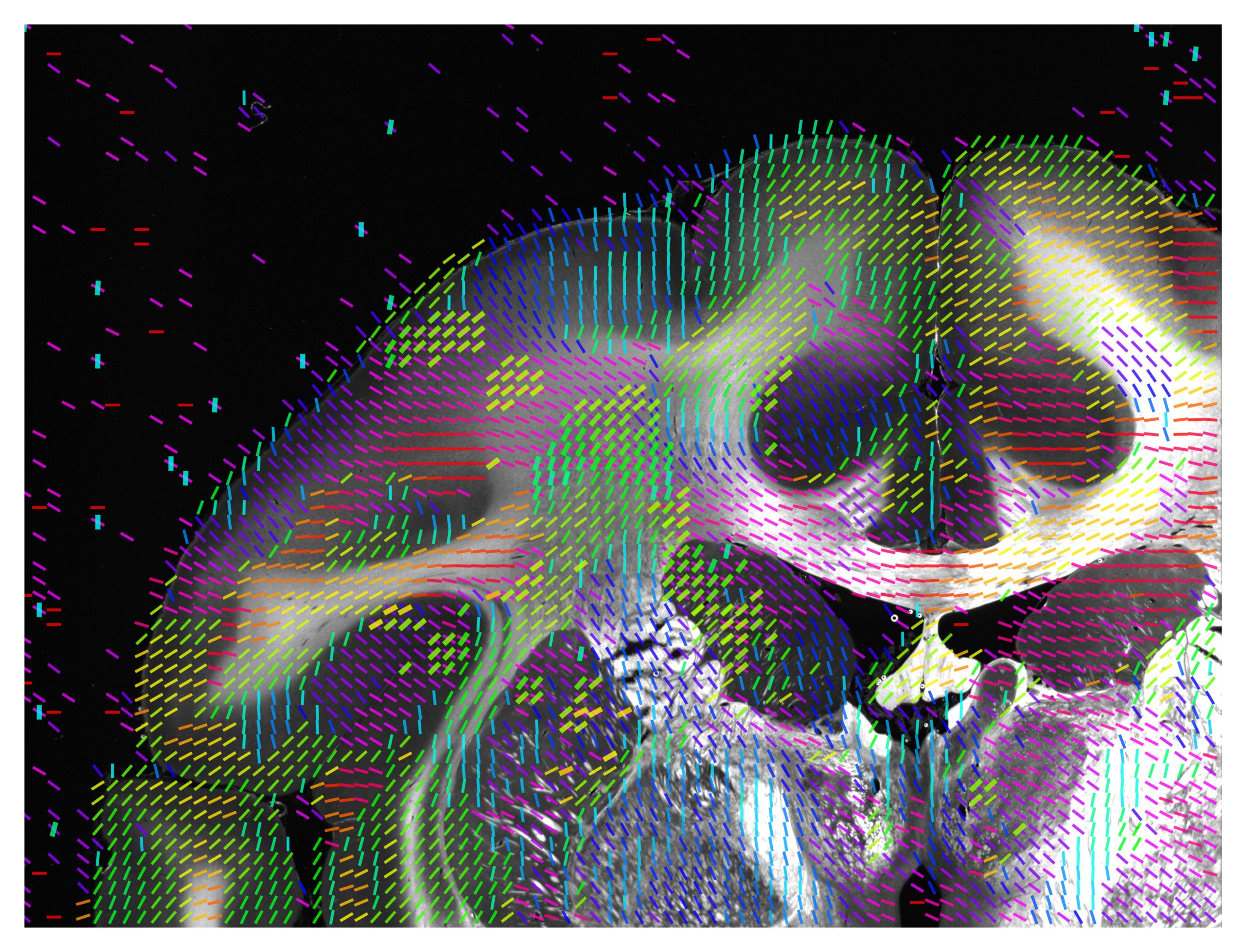
For example, it allows to display the generated parameter maps in different colors, and to show the orientations of (crossing) nerve fibers as colored lines (vector maps) by computing unit vector maps from the direction maps.
The following vector map has been generated with the function visualize_unit_vectors, using alpha = 0.8 (defining the transparency of the background image),
thinout = 20 (i.e. 20 x 20 pixels were evaluated together),
and background_threshold = 0.25 (i.e. if more than 25% of the evaluated pixels are -1, no vector will be computed).
Performance Metrics
The actual runtime depends on the complexity of the SLI image stack. Especially the number of images in the stack and the number of image pixels can have a big influence. To test the performance, one SLI image stack from the coronal vervet brain section (containing 24 images with 2469x3272 pixels each) was analyzed by running benchmark.py. This script will create all parameter maps (non detailed ones in addition to all detailed parameter maps) without any downsampling. All performance measurements were taken without times for reading and writing files. When utilizing the GPU and parameter maps are necessary for further operations, they are kept on the GPU to reduce processing time. The SLI measurement, high prominence peaks and centroids are therefore calculated only once each iteration and are used throughout the whole benchmark. Each benchmark used an Anaconda environment with Python 3.8.5 and all neccessary packages installed.
| CPU | Operating system | With GPU | Time in seconds for this example (8.078.658 pixels) |
|---|---|---|---|
| AMD Ryzen 3700X | Manjaro (Nov 9th 2020) | Disabled | 23.000 ± 1.374 |
| AMD Ryzen 3700X | Manjaro (Nov 9th 2020) | NVIDIA GTX 1070 | 32.013 ± 0.371 |
| AMD Ryzen 3700X | Manjaro (Dez 8th 2020) | NVIDIA RTX 3070 | 22.467 ± 0.370 |
| Intel Core i3-2120 | Ubuntu 18.04 LTS | -N/A- | 86.138 ± 3.57 |
| Intel Core i5-3470 | Ubuntu 20.04 LTS | Disabled | 77.768 ± 6.101 |
| Intel Core i5-3470 | Ubuntu 20.04 LTS | NVIDIA GTX 1070 | 34.169 ± 0.975 |
| Intel Core i5-8350U | Ubuntu 20.10 | -N/A- | 58.945 ± 2.799 |
| Intel Core i7-7820HQ | MacOS Big Sur | -N/A- | 55.709 ± 3.446 |
| 2x Intel Xeon CPU E5-2690 | Ubuntu 18.04 LTS | Disabled | 42.363 ± 3.475 |
| 2x Intel Xeon CPU E5-2690 | Ubuntu 18.04 LTS | NVIDIA GTX 1080 | 27.712 ± 4.052 |
Authors
- Jan André Reuter
- Miriam Menzel
References
 |
Fiber Architecture - INM1 - Forschungszentrum Jülich |
 |
Human Brain Project |
Acknowledgements
This open source software code was developed in part or in whole in the Human Brain Project, funded from the European Union’s Horizon 2020 Framework Programme for Research and Innovation under the Specific Grant Agreement No. 785907 and 945539 ("Human Brain Project" SGA2 and SGA3). The project also received funding from the Helmholtz Association port-folio theme "Supercomputing and Modeling for the Human Brain".
License
This software is released under MIT License
Copyright (c) 2020 Forschungszentrum Jülich / Jan André Reuter.
Copyright (c) 2020 Forschungszentrum Jülich / Miriam Menzel.

Permission is hereby granted, free of charge, to any person obtaining a copy of this software and associated documentation files (the "Software"), to deal in the Software without restriction, including without limitation the rights to use, copy, modify, merge, publish, distribute, sublicense, and/or sell copies of the Software, and to permit persons to whom the Software is furnished to do so, subject to the following conditions:

The above copyright notice and this permission notice shall be included in all copies or substantial portions of the Software.python input parameters -i -o

THE SOFTWARE IS PROVIDED "AS IS", WITHOUT WARRANTY OF ANY KIND, EXPRESS OR IMPLIED, INCLUDING BUT NOT LIMITED TO THE WARRANTIES OF MERCHANTABILITY, FITNESS FOR A PARTICULAR PURPOSE AND NONINFRINGEMENT. IN NO EVENT SHALL THE AUTHORS OR COPYRIGHT HOLDERS BE LIABLE FOR ANY CLAIM, DAMAGES OR OTHER LIABILITY, WHETHER IN AN ACTION OF CONTRACT, TORT OR OTHERWISE, ARISING FROM, OUT OF OR IN CONNECTION WITH THE SOFTWARE OR THE USE OR OTHER DEALINGS IN THE SOFTWARE.
Release history Release notifications | RSS feed


Download files
Download the file for your platform. If you're not sure which to choose, learn more about installing packages.
Source Distribution
Built Distribution
Filter files by name, interpreter, ABI, and platform.
If you're not sure about the file name format, learn more about wheel file names.
Copy a direct link to the current filters
File details
Details for the file SLIX-2.4.2.tar.gz.
File metadata
- Download URL: SLIX-2.4.2.tar.gz
- Upload date:
- Size: 93.2 kB
- Tags: Source
- Uploaded using Trusted Publishing? No
- Uploaded via: twine/4.0.0 CPython/3.9.12
File hashes
| Algorithm | Hash digest | |
|---|---|---|
| SHA256 |
b0fcc20c0eacf2c55226c01131e7ab9b9be390e2f42bf6c8d83aa9058d4d298e
|
|
| MD5 |
6cc74e5e49603046d4329155b4921dd7
|
|
| BLAKE2b-256 |
7b3781ba9c55df78613a02efb3e72bd21a31f6dd0284f2215cd15f01b5b346a9
|
File details
Details for the file SLIX-2.4.2-py3-none-any.whl.
File metadata
- Download URL: SLIX-2.4.2-py3-none-any.whl
- Upload date:
- Size: 79.0 kB
- Tags: Python 3
- Uploaded using Trusted Publishing? No
- Uploaded via: twine/4.0.0 CPython/3.9.12
File hashes
| Algorithm | Hash digest | |
|---|---|---|
| SHA256 |
b1b80422ba5c46a0bcb141ec9c78a689eab61a09ebf362b64777d7168836915b
|
|
| MD5 |
47adfbd6dc9e7ba215421b54d2d227cf
|
|
| BLAKE2b-256 |
e7ef30662008281ae714ec33652e85264328b7e2ad2588844cf9f697102404d0
|


