self organizing maps with periodic boundary conditions

Project description


A simple self-organizing map implementation in Python with periodic boundary conditions.
Self-organizing maps are also called Kohonen maps and were invented by Teuvo Kohonen.[1] They are an unsupervised machine learning technique to efficiently create spatially organized internal representations of various types of data. For example, SOMs are well-suited for the visualization of high-dimensional data.
This is a simple implementation of SOMs in Python. This SOM has periodic boundary conditions and therefore can be imagined as a “donut”. The implementation uses numpy, scipy, scikit-learn and matplotlib.
Installation
som-pbc can be installed from pypi using pip:
pip install som-pbc
To upgrade som-pbc to the latest version, run:
pip install --upgrade som-pbc
Usage
Then you can import and use the SOM class as follows:
import numpy as np
from som import SOM
# generate some random data with 36 features
data1 = np.random.normal(loc=-.25, scale=0.5, size=(500, 36))
data2 = np.random.normal(loc=.25, scale=0.5, size=(500, 36))
data = np.vstack((data1, data2))
som = SOM(10, 10) # initialize a 10 by 10 SOM
som.fit(data, 10000, save_e=True, interval=100) # fit the SOM for 10000 epochs, save the error every 100 steps
som.plot_error_history(filename='images/som_error.png') # plot the training error history
targets = np.array(500 * [0] + 500 * [1]) # create some dummy target values
# now visualize the learned representation with the class labels
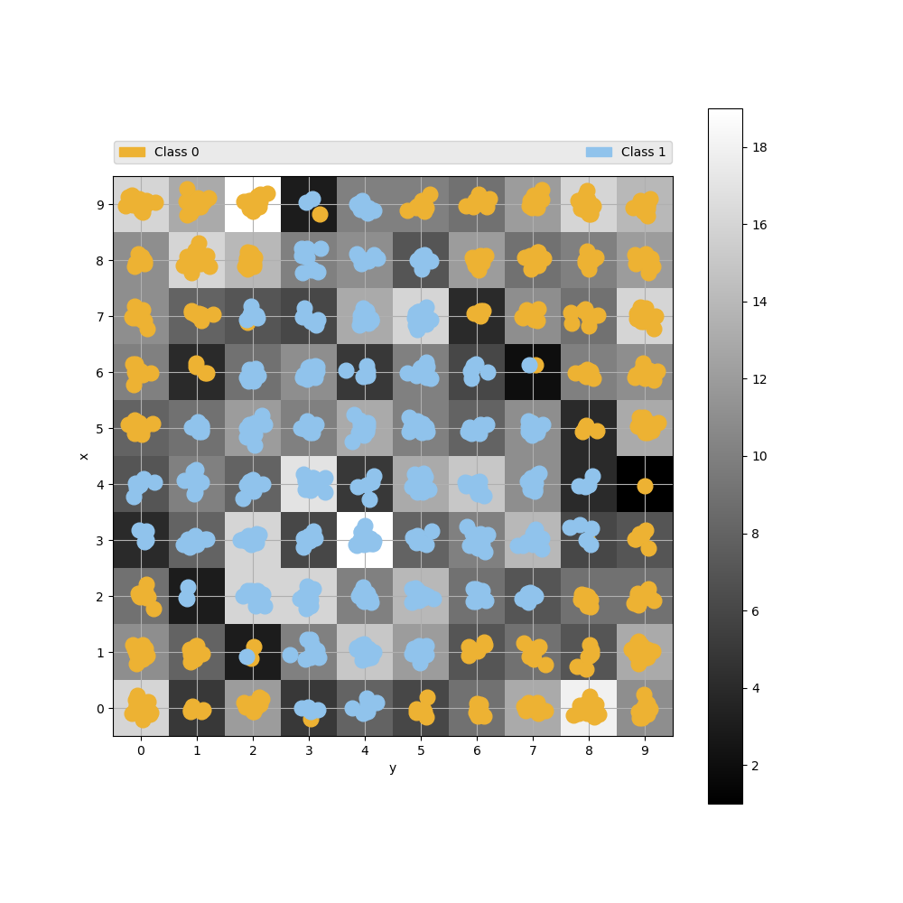
som.plot_point_map(data, targets, ['Class 0', 'Class 1'], filename='images/som.png')
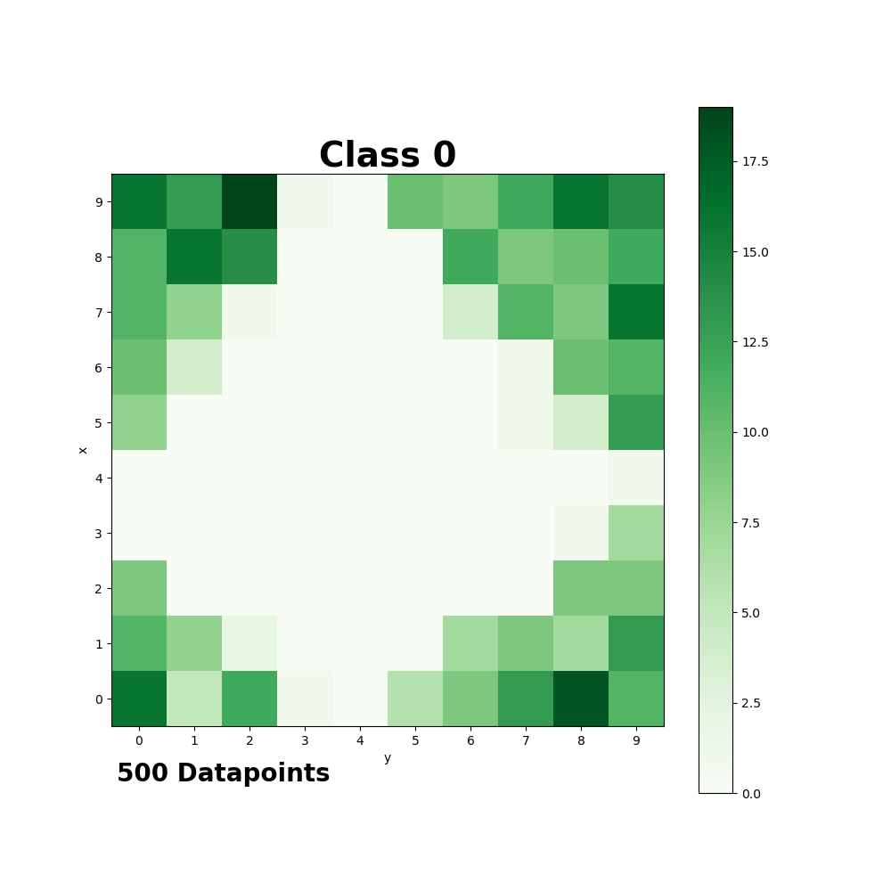
som.plot_class_density(data, targets, t=0, name='Class 0', colormap='Greens', filename='images/class_0.png')
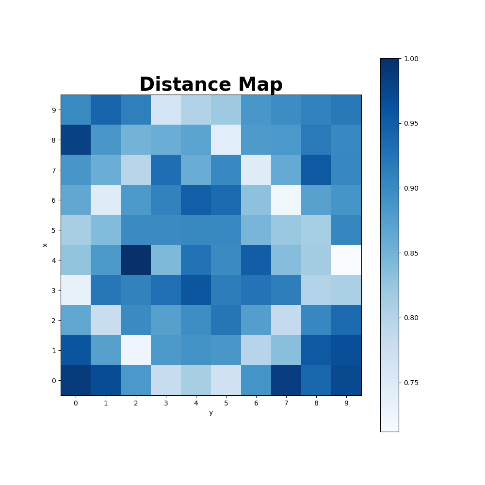
som.plot_distance_map(colormap='Blues', filename='images/distance_map.png') # plot the distance map after training
# predicting the class of a new, unknown datapoint
datapoint = np.random.normal(loc=.25, scale=0.5, size=(1, 36))
print("Labels of neighboring datapoints: ", som.get_neighbors(datapoint, data, targets, d=0))
# transform data into the SOM space
newdata = np.random.normal(loc=.25, scale=0.5, size=(10, 36))
transformed = som.transform(newdata)
print("Old shape of the data:", newdata.shape)
print("New shape of the data:", transformed.shape)Training Error:
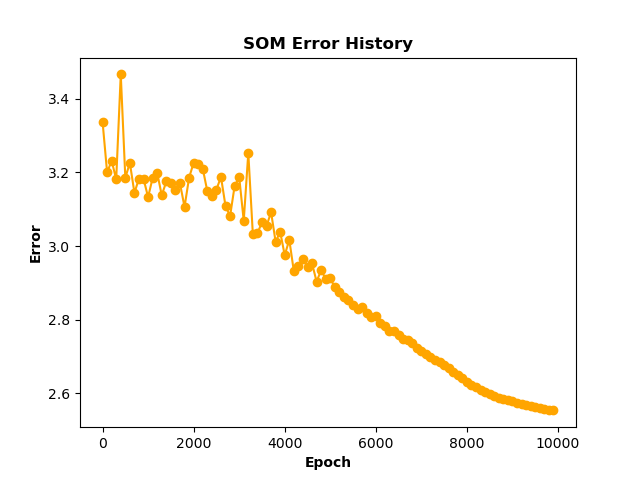
Point Map:
Class Density:
Distance Map:
The same way you can handle your own data.
Methods / Functions
The SOM class has the following methods:
initialize(data, how='pca'): initialize the SOM, either via Eigenvalues (pca) or randomly (random)
winner(vector): compute the winner neuron closest to a given data point in vector (Euclidean distance)
cycle(vector): perform one iteration in adapting the SOM towards the chosen data point in vector
fit(data, epochs=0, save_e=False, interval=1000, decay='hill'): train the SOM on the given data for several epochs
transform(data): transform given data in to the SOM space
distance_map(metric='euclidean'): get a map of every neuron and its distances to all neighbors based on the neuron weights
winner_map(data): get the number of times, a certain neuron in the trained SOM is winner for the given data
winner_neurons(data): for every data point, get the winner neuron coordinates
som_error(data): calculates the overall error as the average difference between the winning neurons and the data
get_neighbors(datapoint, data, labels, d=0): get the labels of all data examples that are d neurons away from datapoint on the map
save(filename): save the whole SOM instance into a pickle file
load(filename): load a SOM instance from a pickle file
plot_point_map(data, targets, targetnames, filename=None, colors=None, markers=None, density=True): visualize the som with all data as points around the neurons
plot_density_map(data, filename=None, internal=False): visualize the data density in different areas of the SOM.
plot_class_density(data, targets, t, name, colormap='Oranges', filename=None): plot a density map only for the given class
plot_distance_map(colormap='Oranges', filename=None): visualize the disance of the neurons in the trained SOM
plot_error_history(color='orange', filename=None): visualize the training error history after training (fit with save_e=True)
References:
[1] Kohonen, T. Self-Organized Formation of Topologically Correct Feature Maps. Biol. Cybern. 1982, 43 (1), 59–69.
This work was partially inspired by ramalina’s som implementation and JustGlowing’s minisom.
Documentation:
Documentation for som-pbc is hosted on readthedocs.io.
Release history Release notifications | RSS feed


Download files
Download the file for your platform. If you're not sure which to choose, learn more about installing packages.
Source Distribution
File details
Details for the file som-pbc-1.0.2.tar.gz.
File metadata
- Download URL: som-pbc-1.0.2.tar.gz
- Upload date:
- Size: 10.6 kB
- Tags: Source
- Uploaded using Trusted Publishing? No
- Uploaded via: Python-urllib/3.7
File hashes
| Algorithm | Hash digest | |
|---|---|---|
| SHA256 |
05f6c1a9976eb4c2cf85d5dfd92853b0e657056347022b4726302f5e8623a238
|
|
| MD5 |
0832cc0f4e860f87282ba1e899262ed0
|
|
| BLAKE2b-256 |
cdb6109919adee957dd89ed8ded78df8293574bcd9161b04bc1b6464d3e5962f
|


