
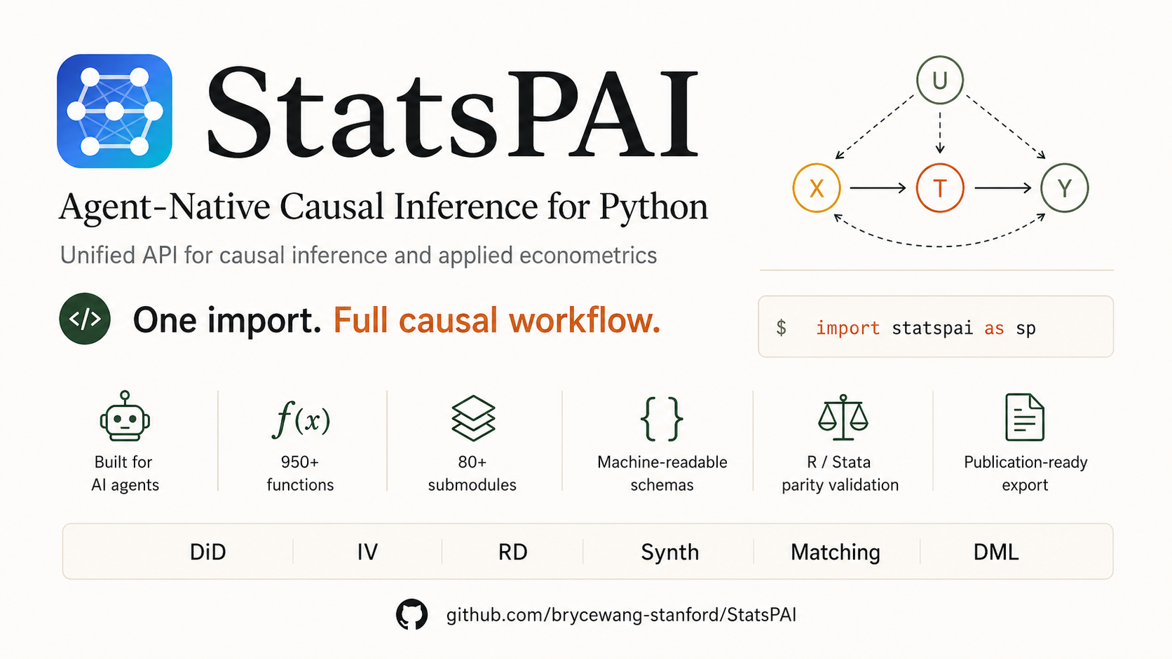
StatsPAI: an Agent&Python-native Stata/R replacement for applied causal inference








StatsPAI is for empirical researchers who would normally jump between Stata, R, and Python. Its goal is to make common Stata/R econometrics and causal-inference workflows feel native in Python: load a dataset, estimate a model, inspect diagnostics, export tables, and hand the result to an agent or notebook without leaving one API.
It is meant to be a practical replacement path for new Python-first work:
- Stata-style routines:
regress,ivregress,reghdfe,csdid,rdrobust,synth,psmatch2,esttab/outreg2. - R-style routines:
lm,fixest,did,rdrobust,Synth,DoubleML,MatchIt,modelsummary,broom. - Stata conventions where they matter:
vce="robust"/vce="cluster firm"onregress,ivregand the likelihood estimators, Stata's small-sample factors and z / t reference distributions,test/lincom/margins, dydx()after any fit, andsp.stata("...", data=df)to run Stata command lines you already have. - Python-native outputs:
.summary(),.tidy(),.plot(),.to_latex(),.to_docx(),.to_agent_summary()where supported by the result object. - Agent-native access: every public function is registered with a
machine-readable schema (
sp.list_functions(),sp.describe_function(),sp.function_schema()), and the bundledstatspai-mcpserver exposes the estimators to MCP clients such as Claude Code, Claude Desktop, and Cursor. - Companion Stata tooling: our own
stata-codecan work with StatsPAI so agents can understand existing Stata workflows, translate them into Python, and cross-check results more smoothly. - Companion skill repos:
Auto-Empirical-Research-Skills,AER-Skills,Awesome-Journal-Skills, andPaper-WorkFlowcan work alongside StatsPAI and an agent as the methods, journal, manuscript, and reproducibility skill layer.
StatsPAI is not a promise that every Stata/R command is bit-for-bit identical.
The API is broad, and the numerical evidence behind it is uneven: some
estimators are checked against R/Stata on identical data, others only against
known-truth simulations, and many are API-stable without a numerical-parity
claim yet. Every function carries a validation_status that says which case
applies: validation_status distinguishes certified/validated evidence from API-stable breadth. See
Validation before relying
on a number for publication.
Install
pip install statspai
Python 3.9 – 3.13. The core install covers estimation, diagnostics, the bundled
datasets, and .xlsx / .docx / LaTeX export. Plotting and heavier backends
are optional extras:
| Extra | Adds | Needed for |
|---|---|---|
statspai[plotting] |
matplotlib, seaborn, plotly | .plot(), sp.ggdid(), sp.interactive() and other figures |
statspai[fixest] |
pyfixest (Python ≥ 3.10) | sp.fixest.* wrappers and the pyfixest cross-validation engine |
statspai[bayes] |
PyMC, ArviZ | Bayesian estimators |
statspai[neural] / statspai[deepiv] |
PyTorch | neural causal models, DeepIV |
statspai[performance] |
JAX | accelerated backends |
statspai[spatial] |
geopandas, libpysal, shapely | shapefile / geometry-based spatial weights |
The interactive figure editor additionally needs ipywidgets inside Jupyter.
import statspai as sp

print(sp.datasets.list_datasets()[["name", "design", "source"]])
StatsPAI bundles 14 datasets that load offline. Most are real published
extracts (source == "bundled CSV"): Card (1995) NLSYM schooling data,
LaLonde/NSW with a PSID comparison group, the U.S. Senate RD data distributed
with R's rdrobust, California Proposition 99, the castle-doctrine panel, and
NHEFS, among others. A few are deterministic simulated replicas calibrated
to a published design (source == "simulated"), including the
Callaway–Sant'Anna mpdta panel used below; their numbers are not the numbers
from the original data.
At a glance: 1,249 registered functions across 87 submodules; 405k LOC (core) + 260k LOC (tests). Run python scripts/registry_stats.py to reproduce these numbers.
If You Come From Stata Or R
| What you used before | Stata / R examples | StatsPAI entry point |
|---|---|---|
| OLS / robust SE | reg y x, vce(robust) / lm() + sandwich |
sp.regress("y ~ x", data=df, vce="robust") |
| Clustered SE | vce(cluster firm) / sandwich::vcovCL(), feols(..., cluster = ~firm) |
vce="cluster firm" (or cluster="firm"); sp.feols(..., cluster="firm") |
| Logit / probit / count models | logit, probit, poisson, nbreg / glm(), MASS::glm.nb() |
sp.logit(), sp.probit(), sp.poisson(), sp.nbreg(), sp.glm() |
| IV / 2SLS | ivregress 2sls / AER::ivreg() |
sp.ivreg("y ~ (d ~ z) + x", data=df) |
| High-dimensional FE | reghdfe / fixest::feols() |
sp.feols("y ~ x | firm + year", data=df) |
| Staggered DiD | csdid / did::att_gt() |
sp.callaway_santanna() + sp.aggte() |
| Regression discontinuity | rdrobust / rdrobust::rdrobust() |
sp.rdrobust() |
| Synthetic control | synth / Synth::synth() |
sp.synth() |
| Matching / PSM | psmatch2 / MatchIt |
sp.psmatch2(), sp.match() |
| Double machine learning | ddml / DoubleML |
sp.dml() |
| Post-estimation | test, lincom, margins, dydx() |
fit.test(), fit.lincom(), sp.margins(fit) |
| Publication tables | esttab, outreg2 / modelsummary |
sp.regtable() |
| Run Stata lines as they are | a .do snippet |
sp.stata("logit y x, vce(cluster id)\nmargins, dydx(x)", data=df) |
| Translate a command | — | sp.from_stata("reghdfe y x, absorb(id year)"), sp.from_r("feols(...)") |
On regress, ivreg, glm, logit, probit, poisson, nbreg, the
ordered / multinomial / conditional logits, the zero-inflated and hurdle
models, liml and more, vce= / robust= follow Stata's vce() grammar
(sp.feols keeps fixest's vcov= / cluster=): True, "robust",
"vce(robust)", "oim", "hc0"–"hc3", and a cluster variable written
inline ("cluster firm", "vce(cluster firm)", "cl firm"). A spelling an
estimator does not implement raises an error instead of quietly falling back
to different standard errors. Robust and cluster SEs apply Stata's
small-sample factors, clustered OLS / IV use t(G-1), and likelihood-based fits
report z. The oim / robust / cluster standard errors of 29 estimators are
pinned to Stata 18 at the 1e-6 parity budget (three documented exceptions
where the two optimisers stop at slightly different points). See the
shared argument grammar guide.
Causal entry points also accept one shared set of argument names next to each
estimator's native spelling: id= for the panel unit, time=,
first_treat= for adoption cohorts, covariates=, and running= /
cutoff= for RD. sp.callaway_santanna(data=mp, y="lemp", time="year", id="countyreal", first_treat="first_treat") is the same call as the
t= / i= / g= version below; a misspelt keyword names the closest one
(runing= → "did you mean 'running'?"), and
sp.describe_function(name)["aliases"] lists the accepted spellings.
sp.esttab(), sp.outreg2(), and sp.modelsummary() still exist, but they are
deprecated thin wrappers over sp.regtable() and emit a DeprecationWarning.
Compared With Other Python Packages
StatsPAI aims to be one broad Stata/R-style workbench. Several focused Python packages do one part of that job, often with a longer track record; if you only need that part, they are good choices.
| Package | What it focuses on | How StatsPAI relates |
|---|---|---|
pyfixest |
fixest-style OLS / IV / GLM with high-dimensional fixed effects, event-study DiD, wild bootstrap, tables | StatsPAI has its own sp.feols (checked against R fixest) and uses pyfixest as an optional wrapper and cross-validation engine. |
linearmodels |
panel models, IV / GMM, system estimation | A core StatsPAI dependency for parts of the panel module, and an independent engine in sp.cross_validate. |
DoubleML |
double/debiased ML (PLR, PLIV, IRM, IIVM), with an R twin | sp.dml is checked against DoubleML on identical learners and folds. |
EconML |
heterogeneous treatment effects: DML, causal forests, DR learners, IV, policy learning | sp.metalearner is checked against EconML's S/T/X learners. |
DoWhy |
graph-based model → identify → estimate → refute workflow; graphical causal models | StatsPAI has DAG and causal-discovery tools, but is estimator-first rather than graph-first. |
CausalPy |
Bayesian-first quasi-experiments in PyMC (plus OLS via scikit-learn): DiD, synthetic control, RD, ITS, IV | StatsPAI centres frequentist econometric conventions (clustered / robust SEs, bias-corrected RD, CS-DiD aggregation) and cross-language parity evidence. |
causallib |
scikit-learn-style IPW, standardization, doubly robust estimation, and causal evaluation | StatsPAI covers these alongside regression, panel, DiD, RD, and synthetic-control workflows in one API. |
Use StatsPAI when you want one package, one function registry, and one agent interface across the everyday Stata/R empirical workflow.
Beginner Examples With Results
The outputs below were produced with StatsPAI 1.29.0 on the bundled
datasets and are pinned by tests/test_readme_examples.py, so they cannot
drift from the code silently. Example 6 uses the Stata vce() grammar and
post-estimation commands introduced in 1.29.0; on an older release install
from source with
pip install "statspai @ git+https://github.com/brycewang-stanford/StatsPAI".
Long summaries are abridged (... marks omitted lines); the numbers are pinned
by tests/test_readme_examples.py and tests/test_synth_placebo_pvalue.py, so
they cannot silently drift from the code again.
1. OLS: the first regress / lm replacement
Question: how much higher is log wage for one more year of schooling in the Card (1995) NLSYM data?
import statspai as sp

card = sp.datasets.card_1995()
ols = sp.regress(
    "lwage ~ educ + exper + expersq + black + south + smsa",
    data=card,
    robust="hc1",
)
print(ols.summary())
Result:
Model: OLS
Method: Least Squares
Dependent Variable: lwage
...
           Coefficient  Std. Error  t-statistic  P>|t|  [0.025  0.975]
Intercept       4.7337      0.0702      67.4718 0.0000  4.5961  4.8712
educ            0.0740      0.0036      20.3208 0.0000  0.0669  0.0812
exper           0.0836      0.0067      12.4165 0.0000  0.0704  0.0968
expersq        -0.0022      0.0003      -7.0443 0.0000 -0.0029 -0.0016
black          -0.1896      0.0174     -10.8781 0.0000 -0.2238 -0.1555
south          -0.1249      0.0154      -8.1339 0.0000 -0.1550 -0.0948
smsa            0.1614      0.0152      10.6374 0.0000  0.1317  0.1912

Model Diagnostics:
--------------------
R-squared           : 0.2905
...
Read it like a Stata/R regression table: conditional on experience, race,
region, and SMSA, one more year of schooling is associated with about 0.074
higher log wage (roughly 7.4%). This is a correlation, not yet a causal return:
schooling is plausibly correlated with unobserved ability, which motivates the
IV in example 2. The HC1 standard errors follow Stata's vce(robust) /
sandwich::vcovHC(type = "HC1") convention.
2. IV / 2SLS: replace ivregress 2sls or AER::ivreg
Question: instrument schooling with growing up near a four-year college
(nearc4).
import statspai as sp

card = sp.datasets.card_1995()
iv = sp.ivreg(
    "lwage ~ (educ ~ nearc4) + exper + expersq + black + south + smsa",
    data=card,
)
print(iv.summary())
Result:
Model: IV-2SLS
Method: Two-Stage Least Squares
Dependent Variable: lwage
...
           Coefficient  Std. Error  t-statistic  P>|t|  [0.025  0.975]
...
educ            0.1323      0.0492       2.6870 0.0072  0.0358  0.2288

Model Diagnostics:
...
First-stage F (educ)        : 16.7176
...
Partial R² (educ)           : 0.0055
Hausman F-stat              : 1.5390
Hausman p-value             : 0.2149
The IV estimate (0.132) is larger than OLS but about 13 times less precise.
The instrument is not strong — nearc4 explains only 0.55% of the residual
variation in schooling (first-stage F ≈ 16.7) — and the Hausman test does not
reject exogeneity of educ (p = 0.21). Default standard errors are the
unadjusted ones with the small-sample correction used by AER::ivreg (Stata:
ivregress 2sls ..., small); pass robust="hc1" for heteroskedasticity-robust
errors, and the first-stage F then uses the same variance estimator, as Stata's
estat firststage does.
With a first stage this modest, report a weak-instrument-robust interval too:
ar = sp.anderson_rubin_ci(
    y="lwage", endog="educ", instruments=["nearc4"],
    exog=["exper", "expersq", "black", "south", "smsa"], data=card,
)
print(ar.summary())
Anderson-Rubin (AR) — weak-IV-robust confidence set
------------------------------------------------------------
  level                : 95%
  grid                 : 401 points on [-0.359, 0.624]
  confidence set       : [0.0384, 0.2612]
3. Staggered DiD: replace csdid or R did
Question: what is the average effect of minimum-wage increases on teen
employment in the Callaway–Sant'Anna mpdta design?
import statspai as sp

mp = sp.datasets.mpdta()   # simulated replica of R did's mpdta
gt = sp.callaway_santanna(
    data=mp,
    y="lemp",
    t="year",
    i="countyreal",
    g="first_treat",
)
overall = sp.aggte(gt, type="simple", bstrap=False)
print(overall.summary())
Result:
==============================================================================
  Callaway and Sant'Anna (2021) — aggte[simple]
==============================================================================

  ATT:      -0.032977 ***
  Std. Error:  (0.007765)
  [95% CI]:    [-0.048195,  -0.017758]
  P-value:     0.0000
...
  Observations:    2,500
...
The aggregated ATT is about -0.033 log points and statistically precise. The
bundled mpdta is a calibrated simulated replica, so this is not the number R
reports on the original mpdta data. What is checked: the same CSV run
through R did::att_gt() + aggte() and Stata csdid returns the same ATT
and standard error (Track A parity module 04_csdid).
4. Regression discontinuity: replace rdrobust
Question: is there a party incumbency advantage at the zero-margin cutoff in U.S. Senate elections?
import statspai as sp

senate = sp.datasets.lee_2008_senate()  # rdrobust's Senate data: x = margin, y = vote share
rd = sp.rdrobust(data=senate, y="y", x="x", c=0)
print(rd.summary())
Result:
==============================================================================
  Sharp RD Estimation
==============================================================================

  RD Effect:       7.506502 ***
  Std. Error:  (1.741258)
  [95% CI]:    [4.093699,  10.919306]
  P-value:     0.0000

------------------------------------------------------------------------------
  Inference
------------------------------------------------------------------------------
      method  estimate     se      z  pvalue  ci_lower  ci_upper
Conventional    7.4141 1.4587 5.0826  0.0000    4.5551   10.2732
      Robust    7.5065 1.7413 4.3110  0.0000    4.0937   10.9193

------------------------------------------------------------------------------
  Observations:    1,297
...
  Bandwidth H:    17.7544
  Bandwidth B:    28.0281
...
  N Effective Left:    360
  N Effective Right:    323
...
The data are the extract of Cattaneo, Frandsen & Titiunik (2015,
doi:10.1515/jci-2013-0010) that ships
with R's rdrobust (the loader keeps its historical name): x is the party's
vote-share margin in the election at time t and y its vote share (0–100) in
the election at t+2, following rdrobust's own illustration. Barely winning at
t raises the vote share at t+2 by about 7.4 percentage points (conventional),
7.5 with robust bias correction; the headline line reports the robust
bias-corrected estimate and CI. On this data
the default MSE-optimal bandwidths, estimates, and standard errors match R
rdrobust::rdrobust() and Stata rdrobust (Track A parity module 06_rd).
Observations are 1,297 because 93 rows have a missing outcome.
5. Synthetic control: replace Stata/R synth
Question: how did California's Proposition 99 affect cigarette sales?
import statspai as sp

prop99 = sp.datasets.california_prop99()
sc = sp.synth(
    data=prop99,
    outcome="cigsale",
    unit="state",
    time="year",
    treated_unit="California",
    treatment_time=1989,
)
print(sc.summary())
Result:
==============================================================================
  Synthetic Control Method
==============================================================================

  ATT:      -19.760529 *
  Std. Error:  (11.233914)
  [95% CI]:    [-41.778595,  2.257538]
  P-value:     0.0769

------------------------------------------------------------------------------
  Detailed Estimates
------------------------------------------------------------------------------
         unit  weight
         Utah  0.3768
      Montana  0.2831
       Nevada  0.1881
  Connecticut  0.0690
New Hampshire  0.0439
     Colorado  0.0391
...
The estimate says California consumed about 20 fewer packs per capita per year
after the intervention. The p-value is the in-space placebo rank: California's
post/pre RMSPE ratio ranks 3rd of the 39 states, so p = 3/39 ≈ 0.077. This
default matches on pre-treatment outcomes only; pass covariates= (e.g.
["lnincome", "retprice", "age15to24", "beer"]) for an ADH-style predictor
specification. That path re-solves the nested V-W problem for every placebo
state and is much slower: pass n_jobs=-1 to fit the placebos in parallel
(bit-identical results), or placebo=False while iterating on the
specification.
Read this number with its caveat, which the full summary also prints:
classical SCM weights are often not uniquely identified on empirical data, and
different correct solvers can land on different donor weights. StatsPAI's
native solver is certified on uniquely identified designs and labelled
identification-dependent elsewhere. On this specification R Synth reaches an
ATT of about -19.59 rather than -19.76; pass backend="synth" (needs a
local R with the Synth package; outcome-lag specification only) when you need
R's exact numbers.
6. Logit, clustered SEs and post-estimation: Stata's logit + margins
Question: in Thornton's Malawi experiment, how much did a randomly offered cash incentive raise the probability that people collected their HIV test results? Villages are the clusters.
import statspai as sp

hiv = sp.datasets.thornton_hiv(complete_case=True)
fit = sp.logit("got ~ any + distvct + male + age", data=hiv,
               vce="cluster villnum")
print(fit.summary())
print(sp.margins(fit, variables=["any"]).round(4))   # margins, dydx(any)
Result:
Model: Logit
Method: Maximum Likelihood (Newton-Raphson)
Dependent Variable: got
...
           Coefficient  Std. Error  z-statistic  P>|z|  [0.025  0.975]
Intercept      -0.6370      0.2010      -3.1691 0.0015 -1.0310 -0.2431
any             2.0178      0.0994      20.3029 0.0000  1.8230  2.2126
distvct        -0.1696      0.0408      -4.1610 0.0000 -0.2496 -0.0897
male           -0.0530      0.1051      -0.5046 0.6139 -0.2590  0.1529
age             0.0100      0.0034       2.9046 0.0037  0.0032  0.0167
...
  variable   dy/dx      se        z  pvalue  ci_lower  ci_upper
0      any  0.3558  0.0145  24.5453     0.0    0.3274    0.3843
As in Stata, the 9 rows with a missing age or village id leave the
estimation sample (N = 2,825, 119 villages); the 4 dropped for a missing
cluster variable are reported in a StatsPAIWarning and in
fit.model_info["n_missing_cluster_dropped"].
The logit coefficient is on the log-odds scale; sp.margins reports what
Stata's margins, dydx(any) reports — the average marginal effect on the
probability, with a delta-method standard error. Being offered any incentive
raised the probability of collecting results by about 36 percentage points.
The coefficients, the village-clustered standard errors, and the marginal
effect match Stata 18 logit ..., vce(cluster villnum) followed by
margins, dydx(any) (0.3558466, SE 0.0144976).
Tests and linear combinations use the full covariance matrix and the fit's own reference distribution (χ² / z here, F / t after OLS):
fit.test("distvct = 0")    # chi2(1) = 17.31, p < 0.001  (Stata: test distvct)
fit.lincom("any + male")   # 1.9648, SE 0.1412           (Stata: lincom any + male)
If you already have the Stata lines, run them as they are:
ame = sp.stata("""
logit got any distvct male age, vce(cluster villnum)
margins, dydx(any)
""", data=hiv)
sp.stata returns the output of the last line — here the same marginal-effects
table. A line it cannot translate faithfully (for example xtreg, fe without
the panel id that xtset would have supplied) raises instead of running a
different model; sp.from_stata(line) shows the Python call without running
it.
Export Results
sp.regtable() is the single table builder behind every format. Build the table
once, then write it wherever your co-authors need it:
import statspai as sp

card = sp.datasets.card_1995()
m1 = sp.regress("lwage ~ educ", data=card, robust="hc1")
m2 = sp.regress("lwage ~ educ + exper + expersq", data=card, robust="hc1")
m3 = sp.regress("lwage ~ educ + exper + expersq + black + south + smsa",
                data=card, robust="hc1")
m4 = sp.ivreg("lwage ~ (educ ~ nearc4) + exper + expersq + black + south + smsa",
              data=card, robust="hc1")

tbl = sp.regtable(
    m1, m2, m3, m4,
    model_labels=["OLS (1)", "OLS (2)", "OLS (3)", "2SLS (4)"],
    coef_labels={"educ": "Years of schooling", "exper": "Experience",
                 "expersq": "Experience squared", "black": "Black",
                 "south": "South", "smsa": "SMSA"},
    drop=["Intercept"],
    title="Returns to Schooling (Card 1995)",
    notes=["HC1 robust SE. Column (4) instruments schooling with nearc4."],
)
print(tbl)                    # terminal
tbl.to_excel("table1.xlsx")   # Excel
tbl.to_word("table1.docx")    # Word
tbl.to_latex()                # LaTeX source; also .to_markdown(), .to_html()
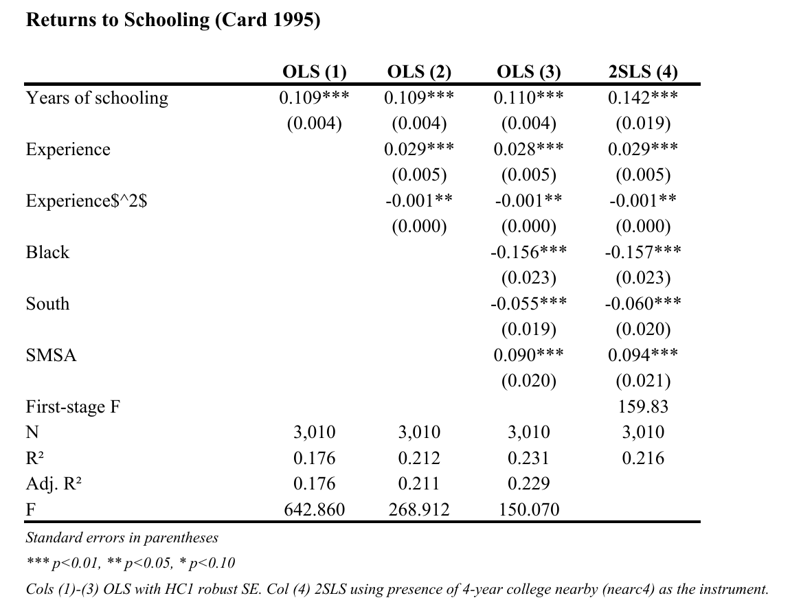
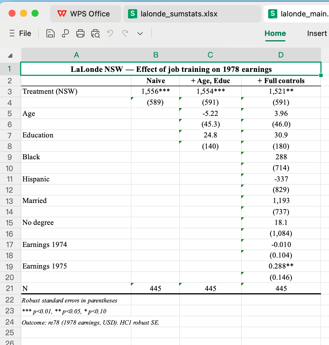
The images are the .xlsx files written by tbl.to_excel(), rendered with
LibreOffice: the Card (1995) table above, and a LaLonde/NSW table regressing
1978 earnings on NSW treatment with a PSID comparison group. The LaLonde table
is also a warning about observational comparisons: the treatment coefficient
moves from -635 to +1,548 once pre-treatment earnings and demographics are
controlled for. See the
export guide for journal
templates, standard-error formats, and single-model exports.
Interactive Plot Editing
If you miss Stata's Graph Editor, use sp.interactive(fig) on any matplotlib
figure returned by StatsPAI. In Jupyter it opens an editing panel next to a
live preview, so beginners can adjust a figure without learning every
matplotlib option first. Requires pip install "statspai[plotting]" ipywidgets.
What it is for:
- change titles, labels, fonts, colors, markers, line widths, grids, legends, axis limits, figure size, and export DPI;
- switch among StatsPAI's publication themes (
academic,aea,minimal,cn_journal) and the built-in matplotlib and seaborn styles; - keep the data layer protected while editing cosmetic elements
(
protect_data=Trueby default); - export reproducible Python code for the edits, so the final figure can be regenerated from a script instead of being only a manual screenshot.
import statspai as sp

mp = sp.datasets.mpdta()
gt = sp.callaway_santanna(data=mp, y="lemp", t="year",
                          i="countyreal", g="first_treat")
agg = sp.aggte(gt, type="dynamic", bstrap=False)
fig, ax = sp.ggdid(agg)

editor = sp.interactive(fig)   # edit the plot in Jupyter
print(editor.generate_code())  # copy reproducible matplotlib edits
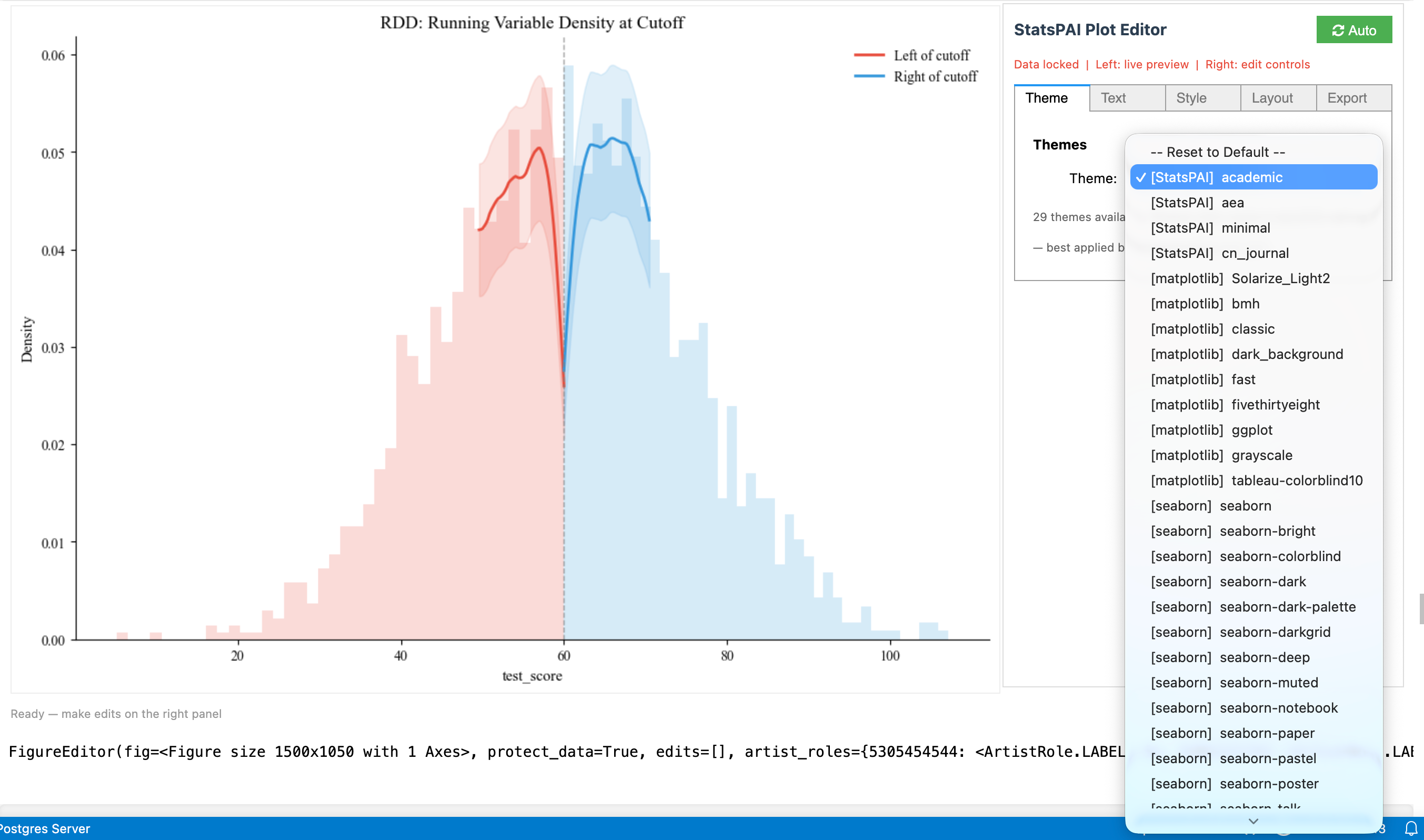
The screenshot above shows the intended workflow: preview on one side, editing controls on the other, and code export for reproducibility.
Everyday Workflow
import statspai as sp

card = sp.datasets.card_1995()
r1 = sp.regress(
    "lwage ~ educ + exper + expersq + black + south + smsa",
    data=card,
    robust="hc1",
)
r2 = sp.ivreg("lwage ~ (educ ~ nearc4) + exper + expersq + black + south + smsa", data=card)

print(r1.summary())                          # human-readable table
print(r1.tidy().head())                      # broom-style dataframe
print(r1.test("black = south"))              # Wald test, like Stata's `test`
print(r1.lincom("black - south"))            # like Stata's `lincom`
tbl = sp.regtable(r1, r2, model_labels=["OLS", "2SLS"])
tbl.to_word("table.docx")                    # Word table
tbl.to_excel("results.xlsx")                 # Excel table
Useful docs:
- Getting started and Cookbook
- Choosing an estimator: DiD, IV, RD, matching, synthetic control
- Migrating: from R, Stata/R command translators, shared argument grammar
- Exporting regression tables
- Agents: agent API, MCP workflow for economists
- Evidence: stability and validation tiers, parity matrix, tier census
Using StatsPAI From An Agent
The same registry that powers sp.help() is exposed three ways.
In Python — discover functions and their schemas without reading source:
import statspai as sp

sp.list_functions(core=True)                   # the ~30 everyday verbs, in order
sp.list_functions(category="causal")[:5]      # names
sp.describe_function("rdrobust")               # parameters, aliases, validation
sp.function_schema("rdrobust")                 # JSON schema for tool calling
sp.from_stata("reghdfe y x, absorb(id year) vce(cluster id)")
# {'tool': 'feols', 'python_code': "sp.feols('y ~ x | id + year', data=df, cluster='id')", ...}
sp.stata("regress y x, vce(cluster id)", data=df)   # translate and run
From the shell — statspai list, statspai describe rdrobust,
statspai search "synthetic control".
Over MCP — the package installs a statspai-mcp stdio server (pure Python,
no extra dependencies). It exposes several hundred estimators and diagnostics as
tools, plus workflow prompts (for example audit_did_result,
stata_command_workflow) and resources such as statspai://catalog. Tools take
a data_path (CSV, Stata .dta, and other formats pandas can read) and return
structured JSON with data provenance. For Claude Code:
claude mcp add statspai -- statspai-mcp
For Claude Desktop, Cursor, and other clients:
{
  "mcpServers": {
    "statspai": { "command": "statspai-mcp", "args": [] }
  }
}
See the MCP workflow guide for data handoff, result handles, and the recommended detect → estimate → audit loop.
Validation: What Has Been Checked, And What Has Not
StatsPAI has a large API surface, so validation status matters.
import statspai as sp

print(sp.describe_function("ivreg")["validation_status"])   # 'certified'
print(sp.list_functions(validation_status="certified")[:5])
Every registered function carries one of these tiers (counts on the current
main; sp.list_functions(validation_status=...) gives the live numbers):
validation_status |
Meaning | Functions |
|---|---|---|
certified |
compared with a named external reference implementation (R, Stata, or the method authors' Python package) on identical inputs, within a pre-registered tolerance | 414 |
validated |
known-truth simulation, published-number, coverage, or documented-convention evidence, but not in the main R/Stata harness | 128 |
api_stable |
stable public interface; unit tests exist, but no numerical-validation claim | 641 |
experimental |
method or API may still change | 3 |
In other words, roughly a third of the registered surface carries numerical evidence today. Breadth is not the same as validation; check the tier of the functions you depend on.
Cross-language parity, made queryable
The tiers above are derived from an auditable parity index: every verified
function records what it was aligned against, to what tolerance, on which test,
and how closely it matched. Each row traces to a committed test artifact (the
pinned StatsPAI ↔ R ↔ Stata harness, version-locked via renv.lock + per-run
provenance) — nothing is asserted from memory.
import statspai as sp

s = sp.parity_status("feols")
print(s)
# feols: bit-exact vs fixest::feols [py/R/Stata] (headline rel_est 5.2e-15 within rel_est<=1e-06, rel_se<=1e-06)
s["reference_versions"]          # {'R': 'R version 4.5.2 (2025-10-31)', 'fixest': '0.14.0'}

sp.parity_summary()              # coverage counts, including the unverified gap
sp.parity_matrix(status="bit-exact")
Grades: bit-exact (headline relative error ≤ 1e-6 against a named R/Stata
reference), aligned (a documented, pre-registered looser tolerance),
analytical-only (recovers a known DGP truth or closed-form identity),
external-replication (reproduces published-paper numbers), and unverified
(registered but no parity evidence attached yet — the honest gap). The full,
auto-generated matrix is published at
docs/parity.md.
For your own data, sp.cross_validate re-runs one estimand through every
independent engine installed locally and reports whether they agree:
card = sp.datasets.card_1995()
cv = sp.cross_validate(card, "iv", y="lwage", endog=["educ"], instruments=["nearc4"],
                       covariates=["exper", "expersq", "black", "south", "smsa"])
print(cv.summary())
Engine              Estimate     Std.Err                95% CI    status
------------------------------------------------------------------------
statspai             0.13229     0.04923      [0.0358, 0.2288]        ok
pyfixest             0.13229     0.04923      [0.0358, 0.2288]        ok
linearmodels         0.13229     0.04923      [0.0358, 0.2288]        ok
R::fixest            0.13229     0.04923      [0.0358, 0.2288]        ok
------------------------------------------------------------------------
VERDICT: ✓ AGREE   (4/4 engines ran)
Engines that are not installed (pyfixest, or R with fixest) are skipped. Every
engine is asked for the same variance estimator (including cluster= and
vcov=) and the same small-sample convention, so the standard errors are
compared as well as the point estimates.
Beyond point-parity, a Track-B coverage study runs B=1000 Monte Carlo
replications per estimator and checks that 95% confidence intervals hit their
nominal rate on known-truth DGPs, against a 99% Wilson acceptance band of
[0.935, 0.967]. The thirteen materialized nominal rows (twelve known-truth DGPs) — OLS on an RCT (0.952),
a 2×2 DiD (0.955), strong-instrument IV (0.962), Callaway–Sant'Anna staggered
ATT (0.947), Sun–Abraham overall ATT (0.950), a two-way FE panel through sp.panel (0.948) and through sp.fast.feols (0.955),
entropy balancing (0.945), a causal-forest AIPW ATE at 2,000 trees (0.959), DML
IRM ATE (0.968), SDID with placebo SEs (0.928), sharp RD with the robust CI
(0.934), and DML PLR with the default learners (0.883) — each also record bias,
Monte Carlo SD and SE calibration. The SDID and RD shortfalls come with
calibrated SEs (RD's intervals equal R rdrobust's draw by draw); the PLR
shortfall is regularisation bias of the default gradient-boosting nuisances
(0.95 with the true nuisances); see tests/coverage_monte_carlo/FINDINGS.md. The committed artifacts live under
tests/coverage_monte_carlo/results_b1000/.
Changelog
Release notes live outside the README:
- CHANGELOG.md for the full version history.
- MIGRATION.md for deprecations and correctness fixes that change numbers.
- Docs changelog page for the rendered documentation site.
The README is intentionally focused on first-time users.
Paper
StatsPAI is described in a peer-reviewed paper in the Journal of Open Source Software (2026, 11(125), 10604): https://doi.org/10.21105/joss.10604. The reviewer-facing material prepared for that review remains the quickest way to audit the package:
Citation
If you use StatsPAI in research, cite the JOSS paper (preferred) and the
underlying method papers for each estimator. sp.citation() returns the paper
citation, sp.citation(which="software") the versioned software entry, and
many result objects expose estimator-level citation helpers.
@article{wang2026statspaijoss,
  author  = {Wang, Biaoyue and Rozelle, Scott},
  title   = {StatsPAI: A Unified, Agent-Native Python Toolkit for
             Causal Inference and Applied Econometrics},
  journal = {Journal of Open Source Software},
  year    = {2026},
  volume  = {11},
  number  = {125},
  pages   = {10604},
  doi     = {10.21105/joss.10604},
  url     = {https://doi.org/10.21105/joss.10604}
}

@software{wang2026statspai,
  author  = {Wang, Biaoyue and Rozelle, Scott},
  title   = {StatsPAI: A Unified, Agent-Native Python Toolkit for
             Causal Inference and Applied Econometrics},
  year    = {2026},
  version = {1.29.0},
  doi     = {10.5281/zenodo.19933900},
  url     = {https://doi.org/10.5281/zenodo.19933900},
  license = {MIT}
}
License
MIT. See LICENSE.
1 maintainer

Release files for StatsPAI 1.31.0
For a detailed explanation of source distributions (sdists) and built distributions (wheels), please see the package formats documentation.
Source distribution (sdist)
| File | Size | Uploaded | |
|---|---|---|---|
| statspai-1.31.0.tar.gz | 23.9 MB | Details |
Built distribution (wheel)
| File | Interpreter | ABI | Platform | Reset |
|---|---|---|---|---|
| statspai-1.31.0-py3-none-any.whl | Python 3 | none | any | Details |
Total release size: 30.1 MB
Release files / statspai-1.31.0.tar.gz
| Download URL | statspai-1.31.0.tar.gz |
|---|---|
| Size | 23.9 MB |
| Tags | Source |
|
SHA-256 checksum How to use checksums |
7b45fa1d275dbbe4b342503e303cef33611d3549b2f2ed45a96ddee309617f8d
|
|
BLAKE2b-256 checksum How to use checksums |
fca6e48c19cdcf802febaff01d439fbac01e0b11b1fc22ef33194f9f5e518a93
|
| Upload date | |
|
Uploaded using Trusted Publishing? What is trusted publishing? |
No |
| Uploaded via |
twine/6.2.0 CPython/3.10.20
|
Release files / statspai-1.31.0-py3-none-any.whl
| Download URL | statspai-1.31.0-py3-none-any.whl |
|---|---|
| Size | 6.2 MB |
| Tags | Python 3 |
|
SHA-256 checksum How to use checksums |
1d915b4a02ec575dd160a456f6d6341cdea4e6d8c532f37076f019affb7651c4
|
|
BLAKE2b-256 checksum How to use checksums |
bb4b5669505d8f29786c2b4558733e57c8e3715b1973f8494be6488b5e94675c
|
| Upload date | |
|
Uploaded using Trusted Publishing? What is trusted publishing? |
No |
| Uploaded via |
twine/6.2.0 CPython/3.10.20
|














