A python library for electrochemical analysis of supercapacitors

Project description

Table of content
Introduction
Welcome to Supycap! This is a Python library for analysis for the Constant Current (CC) curves as well as the Cyclic Voltammetry (CV) curves of two-electrode, symmetrical supercapacitors. It provides an easy and standardised way to quickly extract useful information from the CC and CV data, including the capacitance and the Equivalent Series Resistance (ESR) of the supercapacitor and how they evolve over cycles, with multiple options offered to suit the need of scientific investigations of supercapacitors.
CC analysis
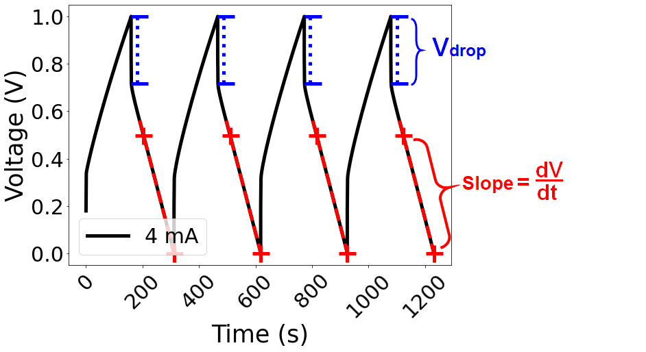
For CC analysis, the capacitance is calculated via linear fitting the second half of the discharging slope in each charging/discharging cycle. For gravimetric capacitance, 


where 


For non-gravimetric capacitance (F):

where I is the current in A and 
The ESR (Ω) is calculated using the voltage drop:

where 
Here is an illustration of how the CC data is analysed:
CV analysis
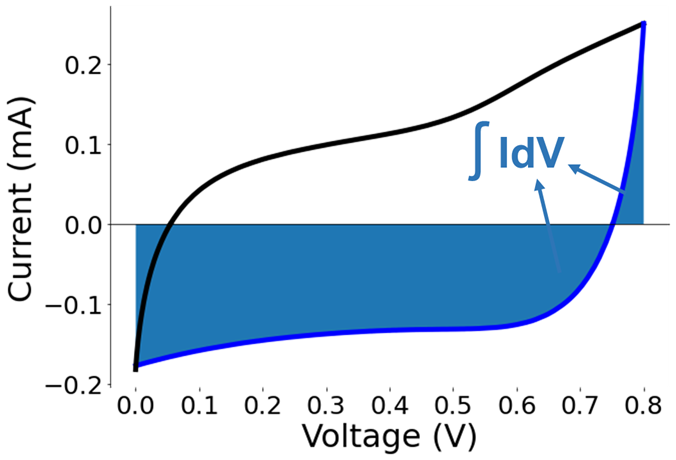
For CV analysis, the capacitance is calculated via integration of the area enclosed by current as the voltage scanned across the potential window. For gravimetric capacitance (

where 


An illustration of how the CV data is analysed is shown below:
Installation
Please follow the instruction under the 'code' tab.
Installation
The library can be downloaded in terminal using the following command:
pip install Supycap
Alternatively, use(https://github.com/AdaYuanChen/Supycap) and follow the instruction under the 'code' tab.
Documentations
This python library offers means to analyse CC data and CV data in the format of text files or csv files, which can be directlt exported from electrochemistry software such as EC Labs. For CC analysis, the program recognises the first data coloumn as time (s) and the second coloumn as voltage (V) by default. For CV analysis, the program recognises the first data coloumn as voltage (V) and the second coloumn as current (mA) by default. However, the optional arguments, such as t_set, V_set, delimeter and row_skip for CC analysis and V_set, I_set, delimeter and row_skip for CV analysis, offers flexibility in dealing with more complex data files which do not meet the default format. For more information, please refer to the documentation for Load_capacitor and CV_analysis, respectively. The documentation includes two parts: CC analysis and CV analysis. CC analysis is further divided into Loading data, which are means for loading data into the Supercap class, and Supercap class, which are methods within the Superclass for extracting data from the analysis.
CC analysis
Loading data
Supercap class
CV analysis
Load_capacitor(pathway, t_set = False, V_set = False, delimiter = False, mass_ls = False, current = False, row_skip = False, ESR_method = True, setting = False, cap_method = False, cap_grav = True)
This function loads the txt/csv file specified on the pathway into the Supercap class ,where capacitance and ESR analysis will be carried out. All relevant information can be extracted from the init function.
Notes
This function supports electrochemical data in either txt or csv format. In a txt file, it is by default that the first coloumn of the file is assumed to be time (s), and the second coloumn is assumed to be Voltage (V) for the CC analysis. The two coloumns are assumed to be seperated by space. However, the optional arguments, t_set, V_set, delimeter and row_skip, offers flexibility in dealing with more complex data files.
Parameters
Arguments
-
pathway : file, str, or pathlib.Path
File, filename of the text file to read. Note that if the library is not allocated in the same directory as the file, the pathway to the file has to be given. Forcurrent=False, current will be directly read from the filename (i.e. the fielname has to include the current followed by'mA'and seperated by'','/'or it is the first component of the filename). If current information cannot be obtained from the filename, the current has be specified via thecurrentargument. For more details, refer to the Examples section. This function currently only supports data in the format of txt or csv. -
t_set : int/str(csv files only), optional
An integer specifying the coloumn index for time(s) data, with the first coloumn being coloumn 0 starting from left. If t_set = False, column 0 will be used as time(s); if t_set = False, there will be prompt asking for time coloumn index to be entered.For csv files, the coloumn index can also be the name of the coloumn (e.g.t_set = 'time(s)'). -
V_set : int/str(csv files only), optional
An integer specifying the coloumn index for voltage(V) data, with the first coloumn being coloumn 0 starting from left. If V_set = False, column 1 will be used as Voltage(V); if t_set = False, there will be prompt asking for voltage coloumn index to be entered. For csv files, the coloumn index can also be the name of the coloumn (e.g.V_set = 'voltage(V)'). -
delimiter : str, optional
A string which is used to seperate the data coloumns in the data file. Ifdelimiter = False, the delimiter is assumed to be space' '. -
mass_ls : list, [[measurements of m1], [measurements of m2]], optional
A list specifying the mass of each electrode in the format as shwon above. Multiple measurements for each electrode should be included for calculation of the uncertainty of the data. All masses should be recorded in mg. If mass_ls = False, a non-gravimetric capacitanc will be calculated and the function returns[[False, False], [False, False]]for the.massesmethod in the resulting Supercap entity (more details for extracting data from the Supercap class in Supercap class>>init -
current : float, optional
Ifcurrent = False, the current value will be directly read from the filename given that it is supplied in the format as specified above in the pathway section. If the current is not included the filename, it should be specified in the form ofcurrent =specified_current. The current value should be recorded in mA. -
row_skip : int, optional
Number of the rows of headers to skip in the txt files. Ifrow_skip = False, row_skip = 1; ifrow_skip = True, a prompt will ask for rows to skip for the file. Enterrow_skip = 0if no rows need to be skipped.
-
ESR_method : int, optional
The method for ESR analysis. It is by default (ESR_method = True) that the ESR analysis will be carried out using method 2 (constant derivative). For all methods available please refer to the next session ESR_method table.ESR_setting = Falsewill return.esr_lsas False in the Supercap class. Available ESR_methods are:ESR_methods = True, False, 1, 101, 2, 201. -
setting : float, optional
ForESR_methods = True, 1, or 2,setting = False. ForESR_methods = 101 or 201, setting is required as the number of points n/second derivative cut off point needed for the constant point method and the constant derivative method, respectively. IfESR_methods = 101 or 201butsetting = False, the function will promt the user to choose a specific value for the ESR analysis before proceeding.
-
cap_method : int, optional
The method for capacitance analysis which determines whether the upper (cap_method = 2) or lower (cap_method = 1) half of the voltage range of the discharging curve will be used. By defaultcap_set = Falseand the program uses the lower half of the discharging curve. For detailed information please refer to the cap_method table below. -
cap_grav : bool, optional
It is by default that the gravimetric capacitance is calculated. By usingcap_grav = Falseormass_ls = False, a non-gravimetric capacitance will be calculated.
ESR_method
| Method | Description |
|---|---|
| True | Default Method 2 |
| False | Returning ESR = False (no ESR calculation) |
| 1 | Default Method 1. dV is calculatied using the voltage difference between the peak voltage and the fourth data point taken after the peak voltage is reached |
| 101 | This method prompts the user to enter an interger n, where dV is determined between the peak voltage and the voltage of the nth points after the peak voltage |
| 2 | Default Method 2. dV is calculatied using the voltage difference between the peak voltage and the smallest data point where the second derivative greater than 0.01 (the second derivative decreases during teh discharging process) |
| 201 | This method prompts the user to enter a float x, where dV is determined between the peak voltage and the voltage of the smallest data point with second derivative over x |
cap_method
| Method | Description |
|---|---|
| False/1 | Default Method. The lower half of the discharging curve is fitted for capacitance calculation. |
| 2 | The upper half of the discharging curve is fitted for capacitance calculation. |
Returns
out: Supercap
A Supercap entity generated from the text file
Examples
>>>supercap1 = Load_capacitor('./CC/3.0_mA_1.0V_010120.txt', ESR_method = 2)
Missing current argument. Please include the current argument in mA:
>>>4
Mass of electrodes absents. Non-gravimetric capacitance is returned
Cycle 1387 has insufficient data points (40% less than average). Skipped for capacitance calculation
>>>supercap1
<Class_Supercap: 4.0 mA, max voltage 1.0 V, 2704 cycle(s), ESR method 2 (setting = 0.01), cap_method 1>
>>>supercap2 = Load_capacitor('./CC/3.0_1.0V_010120.txt', t_set = 0, V_set = 1, mass_ls = [[12,13,12.2], [11, 10.5, 11.6]], current = 4, ESR_method = 2)
>>>supercap2
<Class_Supercap: 4.0 mA, max voltage 1.0 V, 2704 cycle(s), ESR method 2 (setting = 0.01), cap_method 1>
Glob_analysis(path, t_set = False, V_set = False, delimiter = False, mass_ls = False, row_skip = False, ESR_method = True, setting = False, cap_method = False, plot_set = False, plotting = True, save_plot = False)
Loading all txt/csv files in the folder as specified in path. Good for analysing how capacitance changes with current density.
Notes
- Capacitance and ESR analysis for one supercapacitor under different currents.
- Error bars are calculated from the mass errors of the electrodoes as other errors are insignificant compared to that caused by mass.
- The masses in mass_ls is in mg.
- It is assumed that all data files in the folder are measured from the same capacitor, hence they all have the same mass_ls.
- The current has to be included in the file name in the current format as specified under Parameters >> path
Parameters
Arguments
-
path : file, str, or pathlib.Path
File, filename of the text file to read. Note that if the library is not allocated in the same directory as the file, the pathway to the file has to be given. Forcurrent=False, current will be directly read from the filename (i.e. the fielname has to include the current followed by'mA'and seperated by'','/'or it is the first component of the filename). Note that the current values must be recorded in mA.For more details, refer to the Examples section. -
t_set : int/str(csv files only), optional
An integer specifying the coloumn index for time(s) data, with the first coloumn being coloumn 0 starting from left. If t_set = False, column 0 will be used as time(s); if t_set = True, there will be prompt asking for time coloumn index to be entered.For csv files, the coloumn index can also be the name of the coloumn (e.g.t_set = 'time(s)'). -
V_set : int/str(csv files only), optional
An integer specifying the coloumn index for voltage(V) data, with the first coloumn being coloumn 0 starting from left. If V_set = False, column 1 will be used as Voltage(V); if t_set = True, there will be prompt asking for voltage coloumn index to be entered. For csv files, the coloumn index can also be the name of the coloumn (e.g.V_set = 'voltage(V)'). -
delimiter : str, optional
A string which is used to seperate the data coloumns in the data file. Ifdelimiter = False, the delimiter is assumed to be space' '. -
mass_ls : list, [[measurements of m1], [measurements of m2]], optional
A list specifying the mass of each electrode in the format as shwon above. Multiple measurements for each electrode should be included for calculation of the uncertainty of the data. All masses should be recorded in mg. If mass_ls = False, a non-gravimetric capacitanc will be calculated and the function returns[[False, False], [False, False]]for the.massesmethod in the resulting Supercap entity (more details for extracting data from the Supercap class in Supercap class >> init -
row_skip : int, optional
Number of the rows of headers to skip in the txt files. Ifrow_skip = False, row_skip = 1; ifrow_skip = True, a prompt will ask for rows to skip for the file. Enterrow_skip = 0if no rows need to be skipped.
-
ESR_method : int, optional
The method for ESR analysis. It is by default (ESR_method = True) that the ESR analysis will be carried out using method 2 (constant derivative). For all methods available please refer to the next session ESR_method.ESR_setting = Falsewill return.esr_lsas False in the Supercap class. Available ESR_methods are:ESR_methods = True, False, 1, 101, 2, 201. -
setting : float, optional
ForESR_methods = True, 1, or 2,setting = False. ForESR_methods = 101 or 201, setting is required as the number of points n/second derivative cut off point needed for the constant point method and the constant derivative method, respectively. IfESR_methods = 101 or 201butsetting = False, the function will promt the user to choose a specific value for the ESR analysis before proceeding. -
cap_method : bool, optional
The method for capacitance analysis which determines whether the upper (cap_method = 2) or lower (cap_method = 1) half of the voltage range of the discharging curve will be used. By defaultcap_set = Falseand the program uses the lower half of the discharging curve. For detailed information please refer to the cap_method table below. -
plot_set : bool, optional
Figure parameters for plotting. Ifplot_set = False, the defualt settings will be used. Ifplot_set = True, there will be prompts to allow customised settings for plotting. -
plotting : bool, optional
This argument determines whether the capacitance vs. current density plot will be plotted. It is by default thatplotting = True, and the figure will be plotted. Ifplotting = False, the figure will not be plotted. -
save_plot : bool, optional
This argument determines whether the capacitance vs. current density plot will be saved. It is by default thatsave_plot = True, and the figure will be saved as 'Gravimetric specific capacitance vs. current density [datetime].png'. Ifsave_plot = False, the figure will not be saved.
ESR_method
| Method | Description |
|---|---|
| True | Default Method 2 |
| False | Returning ESR = False (no ESR calculation) |
| 1 | Default Method 1. dV is calculatied using the voltage difference between the peak voltage and the fourth data point taken after the peak voltage is reached |
| 101 | This method prompts the user to enter an interger n, where dV is determined between the peak voltage and the voltage of the nth points after the peak voltage |
| 2 | Default Method 2. dV is calculatied using the voltage difference between the peak voltage and the smallest data point where the second derivative greater than 0.01 (the second derivative decreases during teh discharging process) |
| 201 | This method prompts the user to enter a float x, where dV is determined between the peak voltage and the voltage of the smallest data point with second derivative over x |
Returns
out: list
[[list of current density],[list of Supercap objects]]
Examples
>>>CC_glob = Glob_analysis('./various_mA_folder/*.txt', mass_ls=[[10.7, 10.5, 11.0], [11.2, 11.2, 11.5 ]], ESR_method = 2, plotting=False)
>>>CC_glob
([0.0034039334341906206,
  0.011346444780635402,
  0.022692889561270805],
[<Class_Supercap: 0.06 mA, max voltage 0.8 V, 4 cycle(s), ESR method 2 (setting = 0.01), cap_method 1>,
  <Class_Supercap: 0.2 mA, max voltage 0.8 V, 4 cycle(s), ESR method 2 (setting = 0.01), cap_method 1>,
  <Class_Supercap: 0.4 mA, max voltage 0.8 V, 4 cycle(s), ESR method 2 (setting = 0.01), cap_method 1>])
init(self, current, t_V_ls, masses, cap_ls, esr_ls, extrema, cycle_n, m_error, ESR_method, cap_method, faulty_cycles)
Initialize a :class:.Supercap.
Notes
Stores all relevant information for the capacitance/ESR analysis of the supercapacitor. All current values are in mA and mass values are in mg.
Available parameters that can be extracted include:
1. .current
2. .masses
3. .t_ls
4. .V_ls
5. .cap_ls
6. .esr_ls
7. .cycle_n
8. .error
9. .peaks
10. .troughs
11. .esr_method
12. .cap_method
13. .faulty_cycles
The above method follows the name of the Supercap variable. More details in the example section.
Parameters
Arguments
-
current : float
Current at which the CC analysis is undertaken. The current is in mA. -
t_V_ls : list, [[list of time readings], [list of voltage readings]]
The raw data of the CC analysis. -
masses : list, [[average mass of m1, std of m1], [average mass of m2, std of m2]]
The mass measurements for the two electrodes. The mass is in mg. -
cap_ls : list, [list of calculated capacitance for each cycle]
The calculated capacitance for each cycle. -
esr_ls : list, [list of calculated ESR value for each cycle]
The calculated ESR values for each cycle. -
extrema : list, [[peak indices], [trough indices]]
The indices for the peaks and troughs of the voltage readings. -
cycle_n : int
The indices for the peaks and troughs of the voltage readings. -
m_error : list, [list of uncertainties]
The uncertainty for each calculated capacitance value. -
ESR_method : int
The method for ESR analysis. ESR_method = 1/102/2/202 -
cap_method : int
The method for capacitance analysis. cap_method = 1/2 -
faulty_cycles : list, [list of faulty cycle numbers]
A list of cycle numbers (cycle number starting from 1) for the faulty cycles. The faulty cycle could be due to: -
The discharge slope of a CC cycle has significantly more or less data points compared to the neighbouring cycles (more than 50% difference).
-
The discharge slope fails to perform linear fitting.
Examples
>>>supercap1.current #supercap1 is a Supercap class variable.
4.0
>>>supercap1.masses
[[10.2, 0.0912], [12.1, 0.0853]]
repr(self)
Initialize a :class:.Supercap.
Returns
Returns a string which state the current, maximum voltage and number of cycle analysed in the Supercap class.
Examples
>>>Supercap2 #variable as saved in the previous example in Load_capacitor
<Class_Supercap: 4.0 mA, max voltage 1.0 V, 2704 cycle(s), ESR method 2 (setting = 0.01), cap_method 1>
ESR_method_change(self, ESR_method = True, setting = False)
Initialize from a :class:.Supercap.
Notes
Changing the ESR analysis method used for calculating esr_ls.
Parameters
Arguments
-
ESR_method : int, optional
The method for ESR analysis. For all methods available please refer to the next session ESR_method.ESR_setting = Truewill change the ESR analysis method to default, which is the constant second derivative method with a cut-off second derivative of 0.01.ESR_setting = Falsewill turn off the ESR calculation. Available ESR_methods are:ESR_methods = True, False, 1, 101, 2, 201. -
setting : float, optional
ForESR_methods = True, 1, or 2,setting = False. ForESR_methods = 101 or 201, setting is required as the number of points n/second derivative cut off point needed for the constant point method and the constant derivative method, respectively. IfESR_methods = 101 or 201butsetting = False, the function will promt the user to choose a specific value for the ESR analysis before proceeding.
ESR_method
| Method | Description |
|---|---|
| True | Default Method 2 |
| False | Returning ESR = False (no ESR calculation) |
| 1 | Default Method 1. dV is calculatied using the voltage difference between the peak voltage and the fourth data point taken after the peak voltage is reached |
| 101 | This method prompts the user to enter an interger n, where dV is determined between the peak voltage and the voltage of the nth points after the peak voltage |
| 2 | Default Method 2. dV is calculatied using the voltage difference between the peak voltage and the smallest data point where the second derivative greater than 0.01 (the second derivative decreases during teh discharging process) |
| 201 | This method prompts the user to enter a float x, where dV is determined between the peak voltage and the voltage of the smallest data point with second derivative over x |
Returns
out: :class:.Supercap
self.esr_ls
Examples
>>>Supercap2
<Class_Supercap: 4.0 mA, max voltage 1.0 V, 2704 cycle(s), ESR method 2 (setting = 0.01), cap_method 1>
>>>Supercap2.ESR_method_change(ESR_method = 201, setting =1)
The original ESR method is 2 , and the setting is 0.01
array([20.66931875, 20.762845  , 20.72346125, ..., 20.536415  ,
       20.5659475 , 20.570865  ])
>>>Supercap2
<Class_Supercap: 4.0 mA, max voltage 1.0 V, 2704 cycle(s), ESR method 201 (setting = 1), cap_method 1>
Cap_method_change(self, cap_method = False, cap_grav = True, m1 = False, m2 = False)
Initialize from a :class:.Supercap.
Notes
Changing the cap analysis method used for calculating capacitance.
Parameters
Arguments
-
cap_method : int
The method for capacitance analysis into which is changed. Forcap_method = 1 or False), discharge slope of the lower half of the voltage range will be analysed. Forcap_method = 2), discharge slope of the upper voltage range will be analysed. -
cap_grav : bool, optional
It is by default that the gravimetric capacitance is calculated. By usingcap_grav = Falseormass_ls = False, a non-gravimetric capacitance will be calculated. -
m1 : float, optional
The mass of electrode 1 of the supercapacitor. The mass is in mg. -
m2 : float, optional
The mass of electrode 2 of the supercapacitor. The mass is in mg.
Returns
out: :class:.Supercap
self.cap_ls
Examples
>>>Supercap2
<Class_Supercap: 4.0 mA, max voltage 1.0 V, 2704 cycle(s), ESR method 2 (setting = 0.01), cap_method 1>
>>>Supercap2.cap_method_change(cap_method = 2, cap_grav = True)
The original cap_method is 1
The cap_method is changed to 2
Gravimetric capacitance (F g^-1) is being calculated.
Electrode masses are taken as specified previously.
Cycle 1387 has insufficient data points (50% less than average). Skipped for capacitance calculation

array([49.3082373 , 49.37786468, 49.34835958, ..., 51.12061108,
       51.13964009, 51.11665995])

>>>Supercap2.Check_analysis(start = 1387, end = 1389)
Cycle 1387 was skipped for calculation due to errors
>>>Supercap2
<Class_Supercap: 4.0 mA, max voltage 1.0 V, 2704 cycle(s), ESR method 2 (setting = 0.01), cap_method 2>
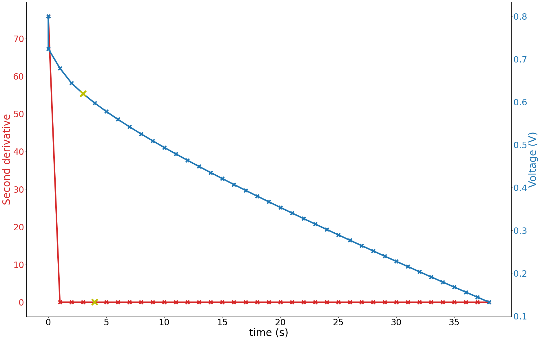
Show_dV2(self, cycle_check = False)
Initialize from a :class:.Supercap.
Notes
Visualising the second derivative and the charge/discharge curve of a specified cycle with the option of changing the ESR analysis method used for calculating esr_ls. It is assumed that ESR_method = 201 is used in this function.
Parameters
Arguments
- Cycle_check : int, optional
The method for ESR analysis. Specify the cycle of the charge/discharge curve and the second derivative to be plotted on the same axes.IfCycle_check = False, the user will be prompted to select a cycle on the CD curve to view as the reference for adjusting the cut off point. (Note: the cycle number starts from 1)
Returns
- A plot of charge discharge curve and the corresponding second derivative
- :class:
.Supercap, optional
self.esr_ls
Examples
>>>Supercap2
<Class_Supercap: 4.0 mA, max voltage 1.0 V, 2704 cycle(s), ESR method 201 (setting = 1), cap_method 1>
>>>Supercap1.Show_dV2()
Of which cycle would you like to see the second derivative? enter a number between 1 and 2704
>>>0
The cut off second derivative currently being used is 1
Are you happy with the cut off point? (yes/no)
>>>no
Please input the value of desired cut off second derivative.
>>>0.01

The cut off second derivative currently being used is 0.01
Are you happy with the cut off point? (yes/no)
>>>yes
Do you wish to change the cut off point to the current value? (setting =0.01)[yes/no]
>>>yes
The original ESR method is 201 , and the setting is 1
>>>Supercap2
<Class_Supercap: 4.0 mA, max voltage 1.0 V, 2704 cycle(s), ESR method 201 (setting = 0.01), cap_method 1>
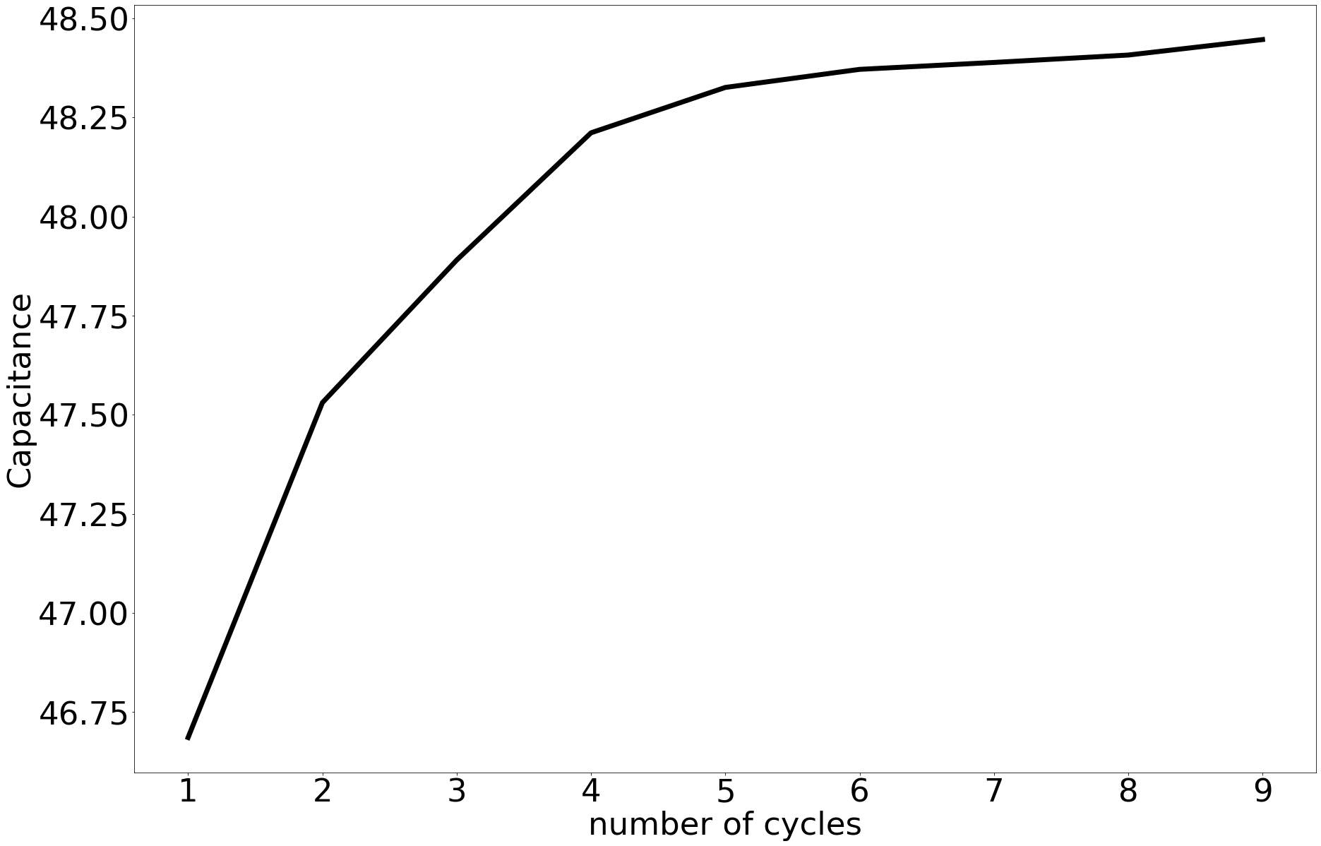
Cap_vs_cycles(self, set_fig=False, save_fig=False)
Initialize from a :class:.Supercap.
Notes
Plotting capacitance against cycle and saving it as 'current mA_cap_vs_cycles_datetime.png'
Parameters
Arguments
-
set_fig : bool, optional
Ifset_fig = True, the user will be prompted to change the setting of the figure. -
save_fig : bool, optional
Ifsave_fig = True, the figure will be saved under the name '[current] mA_cap_vs_cycles_Date[d/m]_Time[h/m].png'
Returns
A figure of capacitance over cycle number
Examples
>>>Supercap1.Cap_vs_cycles(set_fig = True)
Please input length for the figure:
>>>30
Please input width for the figure:
>>>20
Please input the font size for the figure:
>>>45
Please input the line width for the figure:
>>>7
Please input the line colour for the figure:
>>>'black'
Get_info(self)
Initialize from a :class:.Supercap.
Notes
Printing the basic information of the Supercap class
Parameters
Arguments
None
Returns
out::class:string, optional
The number of cycles, the average capacitance, the std of capacitance, the average ESR and its std, the ESR_method and cap_method used.
Examples
>>>Supercap2.Get_info()
The number of cycle(s) analysed is 2704
The number of faulty cycle is 1
The average capacitance is 60.9025 F g^(-1)
The standard deviation of the average is 0.0101
The average ESRs is 14.3174 Ohms
The standard deviation of the ESRs is 0.4699
Lower half of the voltage range in the discharge curve was used for capacitance calculations
Constant second derivative method was used for ESR calculations
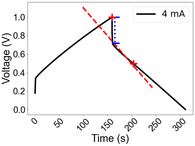
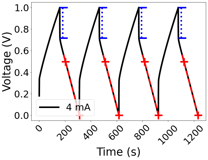
Check_analysis(self, begin = False, end = False, set_fig = False, save_fig = False)
Initialize from a :class:.Supercap.
Notes
Plotting the charge/discharge curve and visualising how the data is analysed (indicate the slope fitting for capacitance and the voltage drop for ESR).
Parameters
Arguments
-
begin : int, optional
The first cycle to be visualised. For
begin = False, the user will be prompted to choose the first cycle to be visualised. Please note that the cycle number starts from 1. -
end : int, optional
The last cycle to be visualised. For
end = False, the user will be prompted to choose the last cycle to be visualised. -
set_fig : bool, optional
Ifset_fig = True, the user will be prompted to change the setting of the figure. -
save_fig : string, optional
For
save_fig=False, the plot will not be saved.For
save_fig=True, the plot will be saved as 'Check_analysis_[datetime].png'.
Returns
A plot of the charge/discharge curve with liniearly fitted slope and voltage drop.
Examples
>>>Supercap1.Check_analysis(begin = 0, end = 4, save_fig = False)
Export(self, name, error = False, delimiter = False)
Initialize a :class:.Supercap.
Notes
Exporting the electrochemical parameters as a txt file
Parameters
Arguments
-
name : str
Name of the exported text file. -
error : bool, optional
Whether a list of uncertainty of capacitance is included. Iferror = False, which is the default setting, a list of uncertainty will not be included; iferror = True, a list of uncertainty will be included. -
delimiter : str, optional
String or character separating columns.
Returns
Returns a text file 'name.txt' including lists of capacitance, ESR and uncertainty of capacitance (optional).
CV_analysis(pathway, m1, m2, scan_r = False, row_skip = False, x_name = False, y_name = False, delimiter = False, int_method = False)
This function loads the txt/csv file specified on the pathway, where capacitance analysis on the Cyclic Voltammetry will be carried out. The function returns a list of capacitance calculated from each CV cycle.
Notes
This function supports electrochemical data in either txt or csv format. In a txt file, it is by default that the first coloumn of the file is assumed to be voltage (V), and the second coloumn is assumed to be current (mA) for the CC analysis. The two coloumns are assumed to be seperated by space. However, the optional arguments, x_name, y_name, delimeter and row_skip, offers flexibility in dealing with more complex data files.
Parameters
Arguments
-
pathway : file, str, or pathlib.Path
File, filename of the text file to read. Note that if the library is not allocated in the same directory as the file, the pathway to the file has to be given. Forscan_r=False, current will be directly read from the filename (i.e. the fielname has to include the current followed by'mvs'and seperated by'','/'or it is the first component of the filename). If scan rate information cannot be obtained from the filename, the scan rate has to be specified via thecurrentargument. For more details, refer to the Examples section. This function currently only supports data in the format of txt or csv. -
m1 : float, optional
The mass of electrode 1 of the supercapacitor. The mass is in mg. -
m2 : float, optional
The mass of electrode 2 of the supercapacitor. The mass is in mg. -
scan_r : float, optional
Ifscan_r = False, the scan rate value in mV/s will be directly read from the filename given that it is supplied in the format as specified above in the pathway section. If the current is not included the filename, it should be specified in the form ofscan_r =specified_scan_rate -
row_skip : int, optional
Number of the rows of headers to skip in the txt files. Ifrow_skip = False, row_skip = 1; ifrow_skip = True, a prompt will ask for rows to skip for the file. Enterrow_skip = 0if no rows need to be skipped. -
V_set : int/str(csv files only), optional
An integer specifying the coloumn index for voltage in V, with the first coloumn being coloumn 0 starting from left. Ifx_name = False, column 0 will be used as voltage(V); if x_name = True, there will be prompt asking for scan rate coloumn index to be entered.For csv files, the coloumn index can also be the name of the coloumn (e.g.x_name = 'voltage(V)'). -
I_set : int/str(csv files only), optional
An integer specifying the coloumn index for voltage(V) data, with the first coloumn being coloumn 0 starting from left. Ify_name = False, column 1 will be used as current in mA; if y_name = True, there will be prompt asking for current coloumn index to be entered. For csv files, the coloumn index can also be the name of the coloumn (e.g.I_set = 'current(mA)'). -
delimiter : str, optional
A string which is used to seperate the data coloumns in the data file. Ifdelimiter = False, the delimiter is assumed to be space' '.
-
int_method : int, optional
The method for integration of the enclosed area. It is by default (int_method = False) that the area under the curve will be calculated using the Simpson's rule. For all methods available please refer to the next session int_method table. -
calc_method : int, optional
The method which determines whether capacitance or capacity (enclosed area divided by mass) is being calculated. Ifcalc_method = 1, capacitance is calculated; ifcalc_method = 2, capacity is calculated by dividng the enclosed area by the mass of the electrodes.
int_method
| Method | Description |
|---|---|
| False or 1 | Default method. Integration using the Simpson's rule and integrates over discharging curve only. |
| 101 | Integration using the Simpson's rule and integrates over both the charging and discharging curves. |
| 2 | Integration using the trapezoidal rule and integrates over discharging curve only. |
| 202 | Integration using the trapezoidal rule and integrates over both the charging and discharging curves. |
Returns
out: [list of calculated gravimetric capacitance]
Examples
>>>CV_analysis('../cell1_CV/1.2V_CA2.csv', m1=10, m2=9, scan_r=1, x_name = 'voltage', y_name ='current',delimeter=',', int_method=1)
4  CV cycles are being analysed using integration method 1
[86.30233646681373, 88.433682993075, 89.45296144982, 90.0191569583757]
Release history Release notifications | RSS feed


Download files
Download the file for your platform. If you're not sure which to choose, learn more about installing packages.
Source Distribution
File details
Details for the file Supycap-2.2.tar.gz.
File metadata
- Download URL: Supycap-2.2.tar.gz
- Upload date:
- Size: 43.6 kB
- Tags: Source
- Uploaded using Trusted Publishing? No
- Uploaded via: twine/3.2.0 pkginfo/1.5.0.1 requests/2.22.0 setuptools/41.4.0 requests-toolbelt/0.9.1 tqdm/4.36.1 CPython/3.7.4
File hashes
| Algorithm | Hash digest | |
|---|---|---|
| SHA256 |
03904b14f415d404dd7ae0d32e86722fc9a5f3025e3f07cd616873fa1a4bf545
|
|
| MD5 |
a24ff569ad7abd741cc2599a1a390a9f
|
|
| BLAKE2b-256 |
7f350e233c38adc4406c58fef4418608b4a831464880b0af1769290afe630735
|


