A package for TensorConvolution+ distribution network aggregated flexibility area estimation

Project description
I. Acknowledgements
The authors are part of the IEPG group and AI Energy lab of TU Delft. This research is part of the research program ‘MegaMind - Measuring, Gathering, Mining and Integrating Data for Self-management in the Edge of the Electricity System’, (partly) financed by the Dutch Research Council (NWO) through the Perspectief program under number P19-25.


II. Package
The proposed package includes the functionalities to perform flexibility area estimation.
To install the package through a file, place the tensorconvolutionplus-0.1.0.tar.gz file in an accessible path and run:
(.venv) $ pip install path/to/package/tensorconvolutionplus-0.1.0.tar.gzTo install the package online (currently unavailable), run:
(.venv) $ pip install tensorconvolutionplusMain functionalities include:
- TensorConvolution+, estimating FAs using the TensorConvolution+ algorithm. In the current version, the estimations can vary in:
Pandapower network (names) for MV Oberrhein0, MV Oberrhein1, Cigre MV. If another network is in similar format as these pandapower networks, it can also be an input instead.
Resolutions for the discretization of the flexibility resources.
Network voltage and loading constraints.
Voltage and loading sensitivity thresholds.
Including/Excluding FSPs only offering full output reductions, or limited setpoints ( including these FSPs currently uses the numpy library and not pytorch).
Flexibility service providers.
Network structure and initial operating conditions.
- Shape of flexibility resources. Currently FSP limits are:
the output cannot exceed the maximum apparent power of the FSP (resulting in a semi-oval shape),
the output P cannot exceed the maximum apparent power of the FSP, the output abs(Q) cannot exceed the maximum apparent power of the FSP (resulting in rectangular shape).
additional shapes can be adopted by modifying the sample generation function (not impacting the TensorConvolution+ aggregation).
- TensorConvolution+, while storing estimated tensors and other useful information to adapt flexibility areas for different operating conditions. In the current version, the estimations can vary in:
Pandapower network (names) for MV Oberrhein0, MV Oberrhein1, Cigre MV. If another network is in similar format as these pandapower networks, it can also be an input instead.
Resolutions for the discretization of the flexibility resources.
Network voltage and loading constraints.
Voltage and loading sensitivity thresholds.
Flexibility service providers.
Network structure and initial operating conditions.
- Shape of flexibility resources. Currently FSP limits are:
the output cannot exceed the maximum apparent power of the FSP (resulting in a semi-oval shape),
the output P cannot exceed the maximum apparent power of the FSP, the output abs(Q) cannot exceed the maximum apparent power of the FSP (resulting in rectangular shape).
additional shapes can be adopted by modifying the sample generation function (not impacting the TensorConvolution+ aggregation).
- TensorConvolution+, while loading previously estimated tensors and other useful information to adapt flexibility areas from prior different operating conditions. In the current version, the estimations can vary in:
Pandapower network (names) for MV Oberrhein0, MV Oberrhein1, Cigre MV. If another network is in similar format as these pandapower networks, it can also be an input instead. The network must be the same as the stored one.
Resolutions for the discretization of the flexibility resources. Must be the same as the stored simulation.
Network voltage and loading constraints.
Flexibility service providers. Must be the same as the stored simulation.
Network structure and initial operating conditions.
Shape of flexibility resources. Must be the same as the stored simulation.
- Monte Carlo power flow based flexibility area estimation. In the current version, the estimations can vary in:
Pandapower network (names) for MV Oberrhein0, MV Oberrhein1, Cigre MV. If another network is in similar format as these pandapower networks, it can also be an input instead.
Network voltage and loading constraints.
Number of samples.
- Distribution used for samples, including:
‘Hard’: Exploring the limit from each resource flexibility.
‘Uniform’: Applying uniform distribution.
‘Kumaraswamy’: Applying the Kumaraswamy distribution.
Flexibility service providers.
Including/Excluding FSPs only offering full output reductions, or limited setpoints (including these FSPs currently uses the numpy library and not pytorch).
Network structure and initial operating conditions.
- Exhaustive power flow based flexibility area estimation. In the current version, the estimations can vary in:
Pandapower network (names) for MV Oberrhein0, MV Oberrhein1, Cigre MV. If another network is in similar format as these pandapower networks, it can also be an input instead.
Network voltage and loading constraints.
Resolutions for the discretization of the flexibility resources.
Flexibility service providers.
Including/Excluding FSPs only offering full output reductions, or limited setpoints (including these FSPs currently uses the numpy library and not pytorch).
Network structure and initial operating conditions.
- Optimal power flow based flexibility area estimation. In the current version, the estimations can vary in:
Pandapower network. Cigre MV in radial structure converges whereas alternative networks might fail to converge.
Network voltage and loading constraints. Transformer loading is excluded due to convergence issues.
Flexibility service providers.
Network structure and initial operating conditions.
III. Examples
All main functionalities require first importing the FA_Estimator script from the package. Therefore, all the following examples start with the Python line:
from TensorConvolutionPlus import FA_Estimator as TCPIII.A) Monte Carlo Power Flow
This section includes examples using the Monte Carlo PF estimation functionality. These examples used the Python script code:
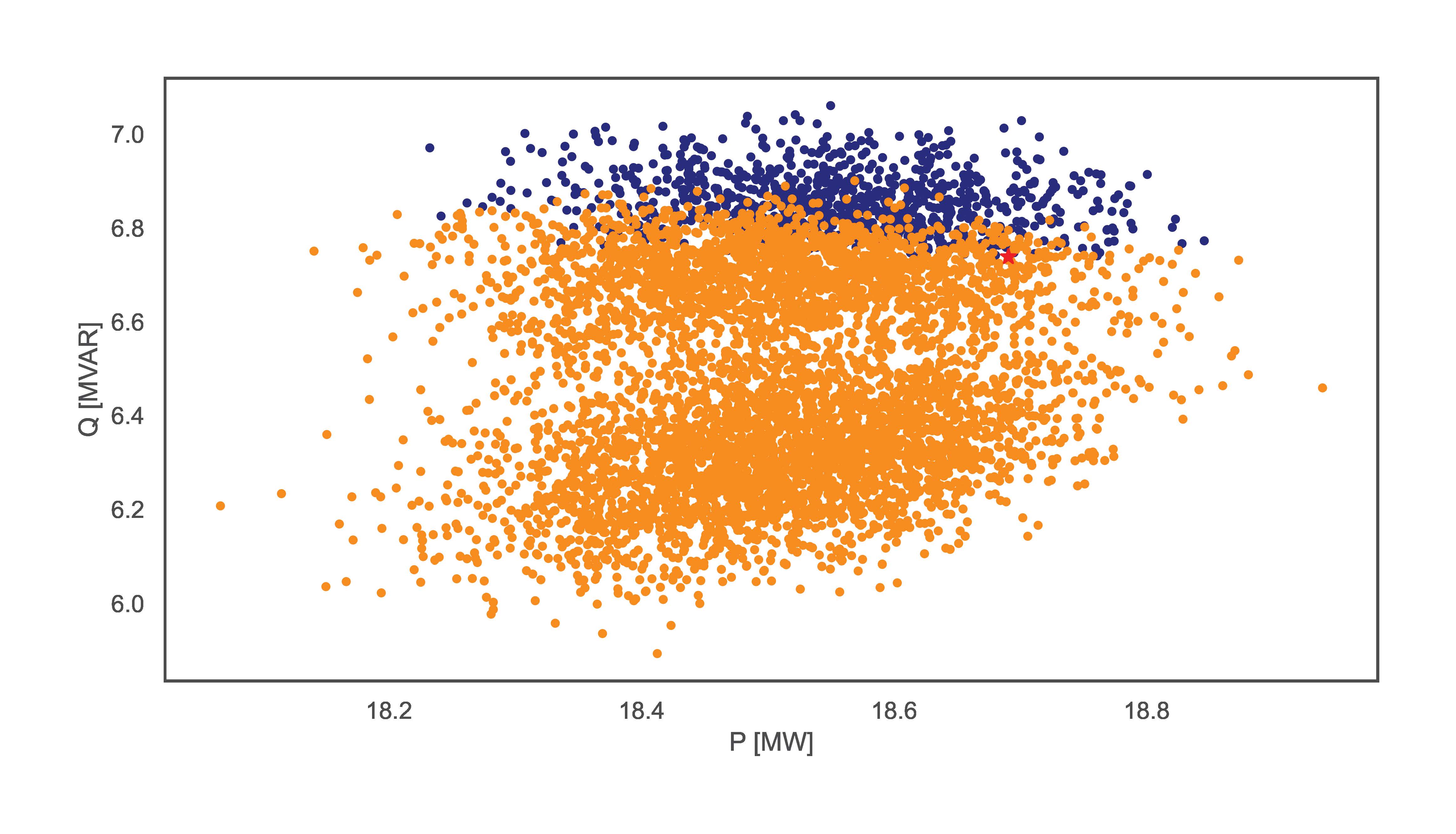
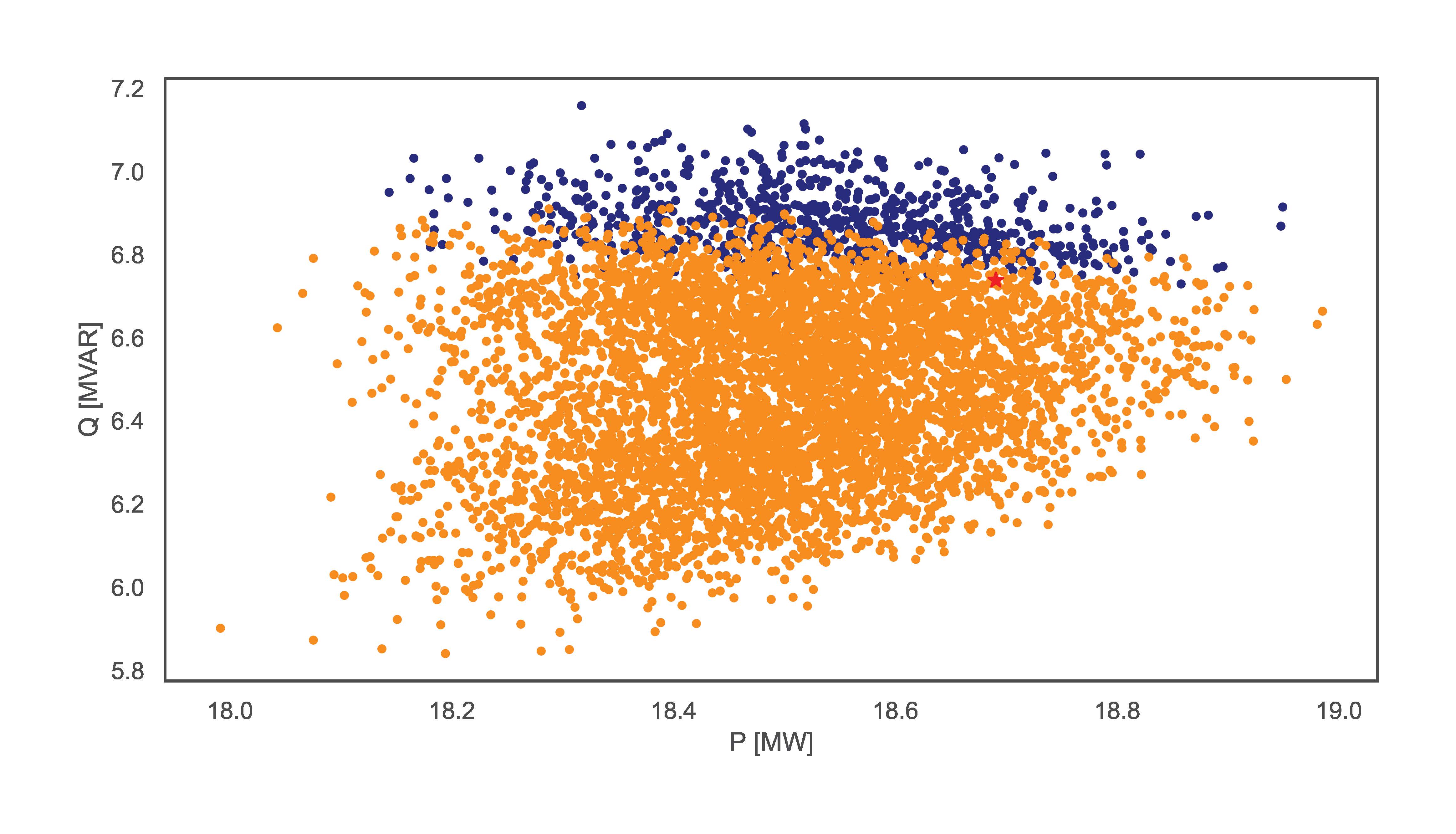
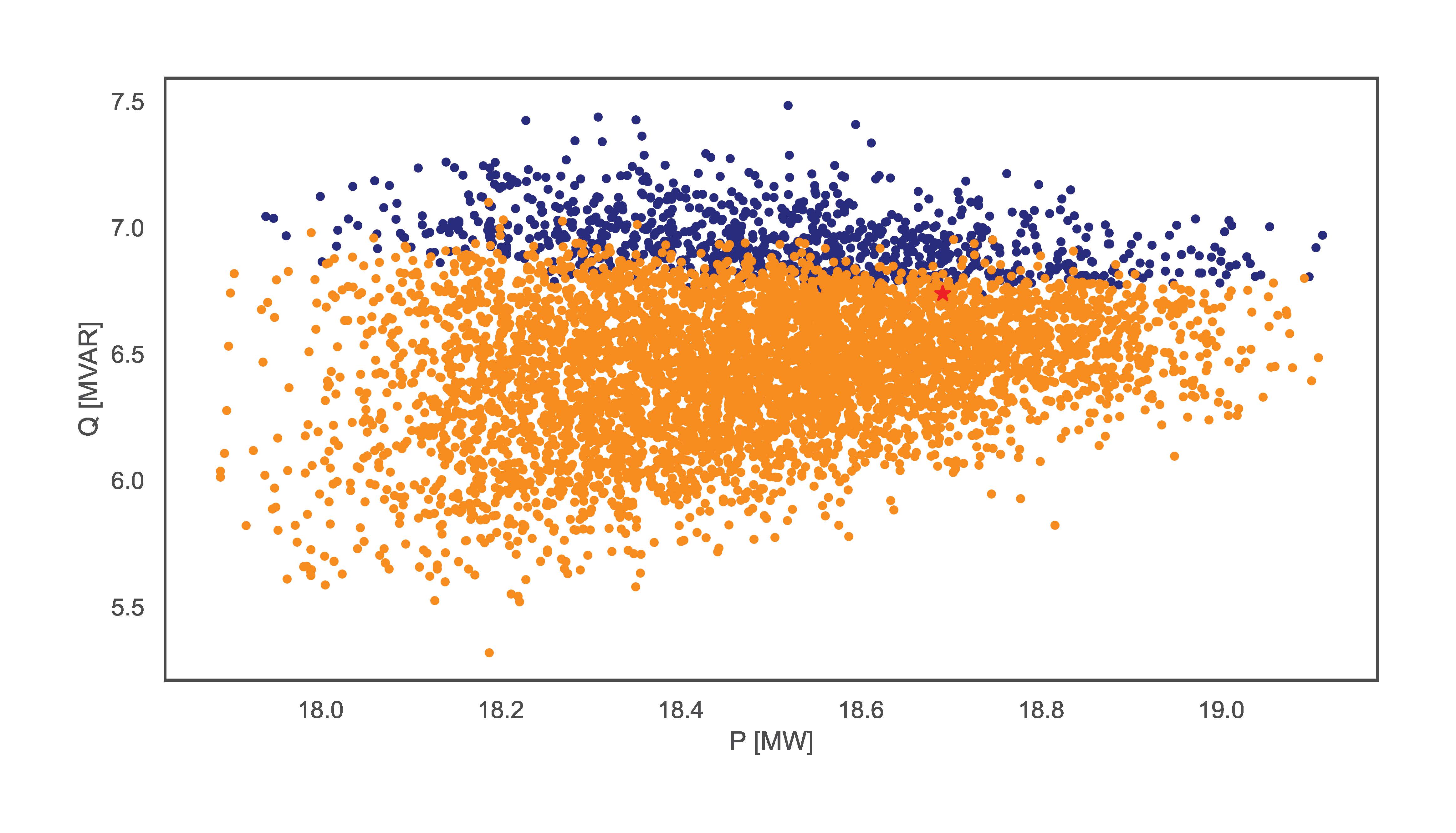
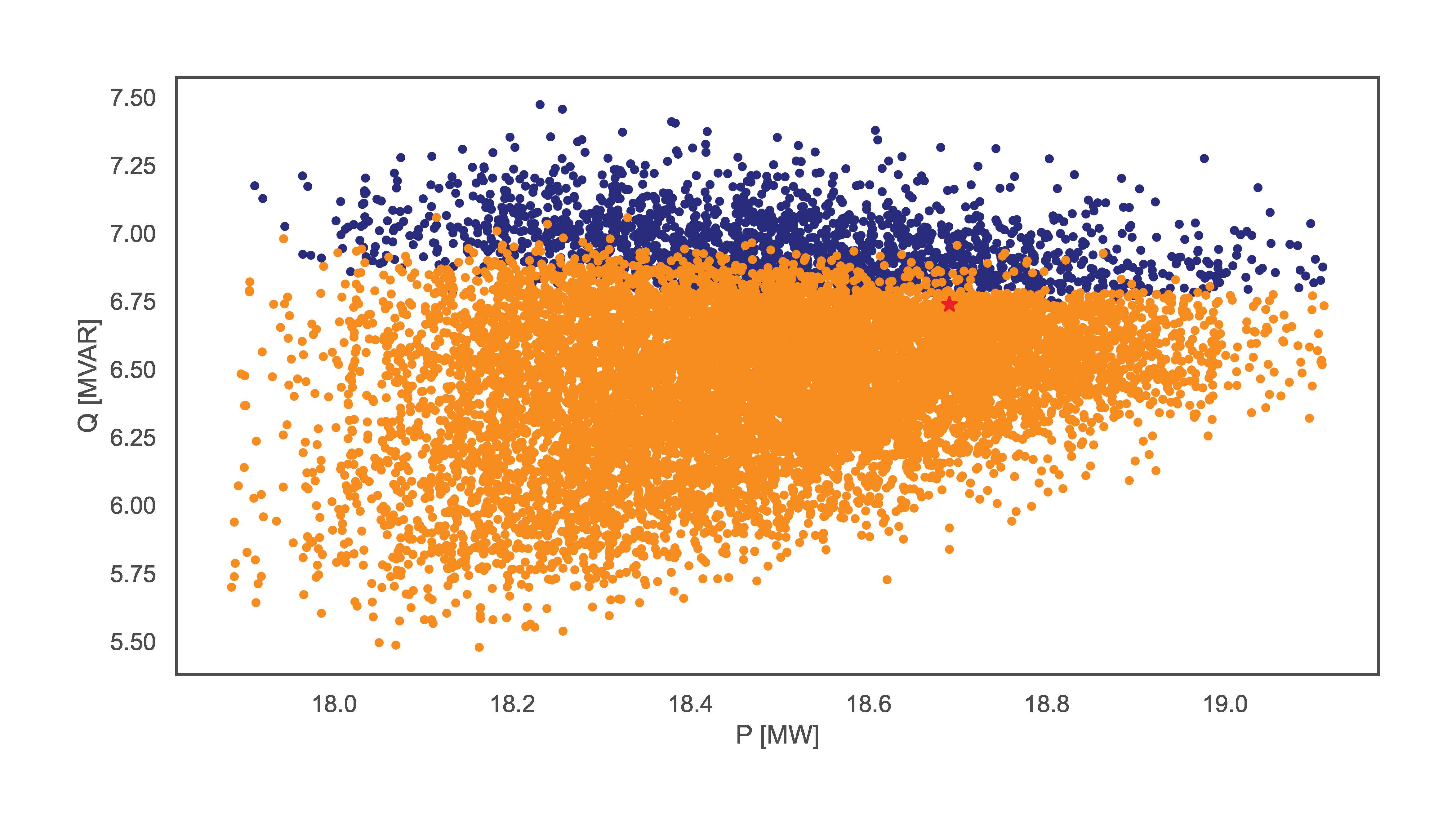
TCP.monte_carlo_pf(net_name='MV Oberrhein0', no_samples=6000, fsp_load_indices=[1, 2, 3], fsp_dg_indices=[1, 2, 3], distribution='Uniform')

TCP.monte_carlo_pf(net_name='MV Oberrhein0', no_samples=6000, fsp_load_indices=[1, 2, 3], fsp_dg_indices=[1, 2, 3], distribution='Kumaraswamy')

TCP.monte_carlo_pf(net_name='MV Oberrhein0', no_samples=6000, fsp_load_indices=[1, 2, 3], fsp_dg_indices=[1, 2, 3])

TCP.monte_carlo_pf(net_name='MV Oberrhein0', no_samples=12000, fsp_load_indices=[1, 2, 3], fsp_dg_indices=[1, 2, 3])
The examples vary in sampling distribution and number of samples. The figures bellow illustrate the resulting FA for each line respectively. The lines without distribution input automatically obtain the ‘Hard’ distribution.
III.B) Exhaustive Power Flow
This section includes examples using the exhaustive power flow-based functionality. The script for the examples is:
TCP.exhaustive_pf(net_name='MV Oberrhein0', dp=0.15, dq=0.3, fsp_load_indices=[1, 2, 3], fsp_dg_indices=[1, 2, 3])

TCP.exhaustive_pf(net_name='MV Oberrhein0', dp=0.01, dq=0.02, fsp_load_indices=[5], fsp_dg_indices=[5])
The examples vary in resolution and number of FSPs. The figures bellow illustrate the resulting FA for each line respectively.
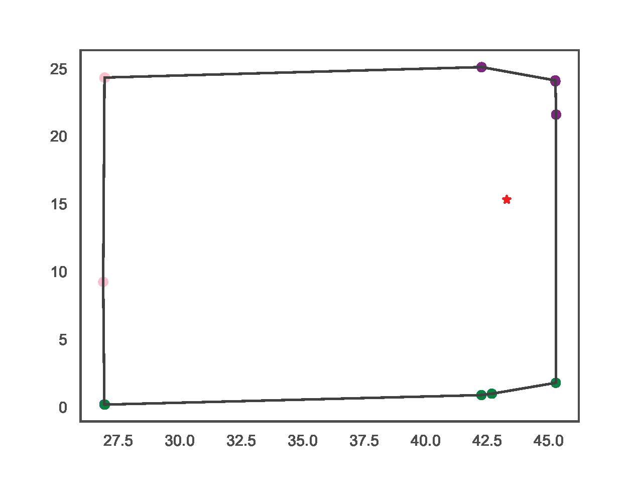
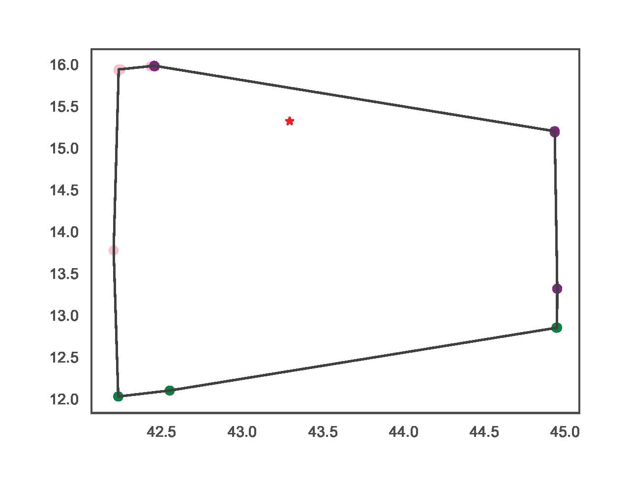
III.C) Optimal Power Flow
This section illustrates examples using the OPF estimation functionality. These examples used the Python script code:
TCP.opf(net_name='CIGRE MV', opf_step=0.1, fsp_load_indices=[3, 5, 8], fsp_dg_indices=[8])

TCP.opf(net_name='CIGRE MV', opf_step=0.1, fsp_load_indices=[1, 4, 9], fsp_dg_indices=[8])
The examples vary in FSPs. The figures bellow illustrate the resulting FA for each line respectively.
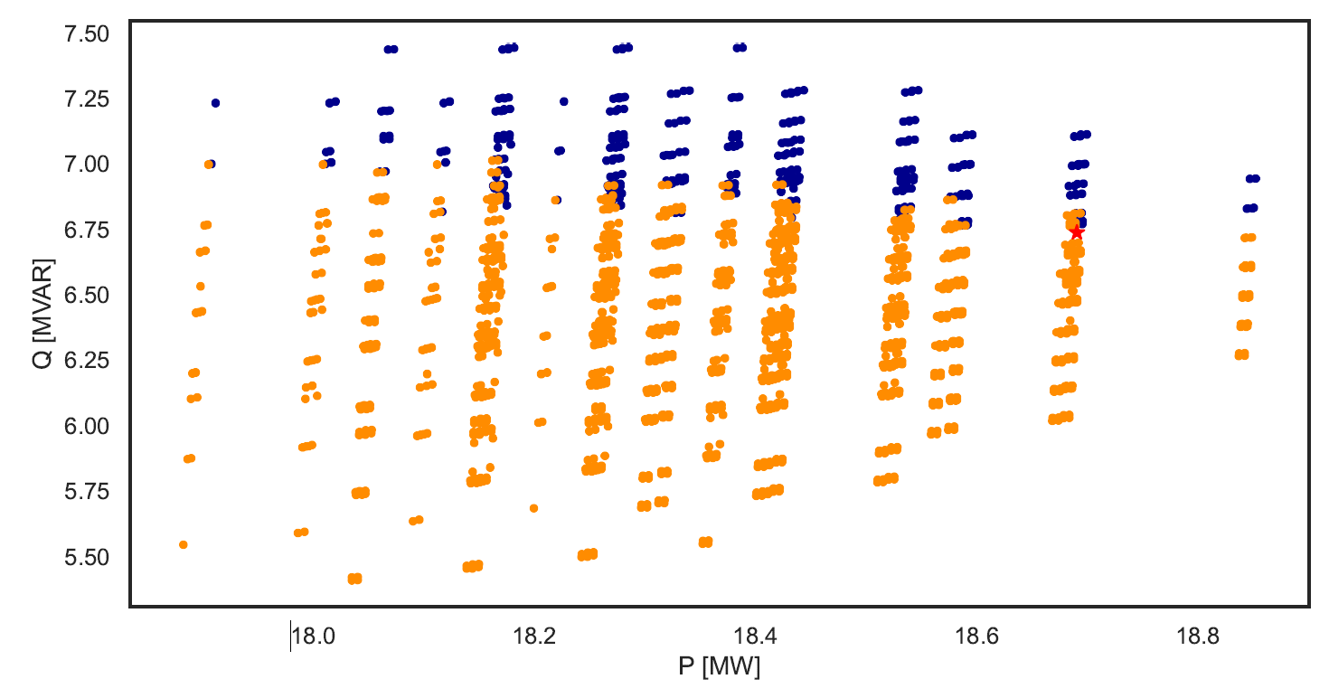
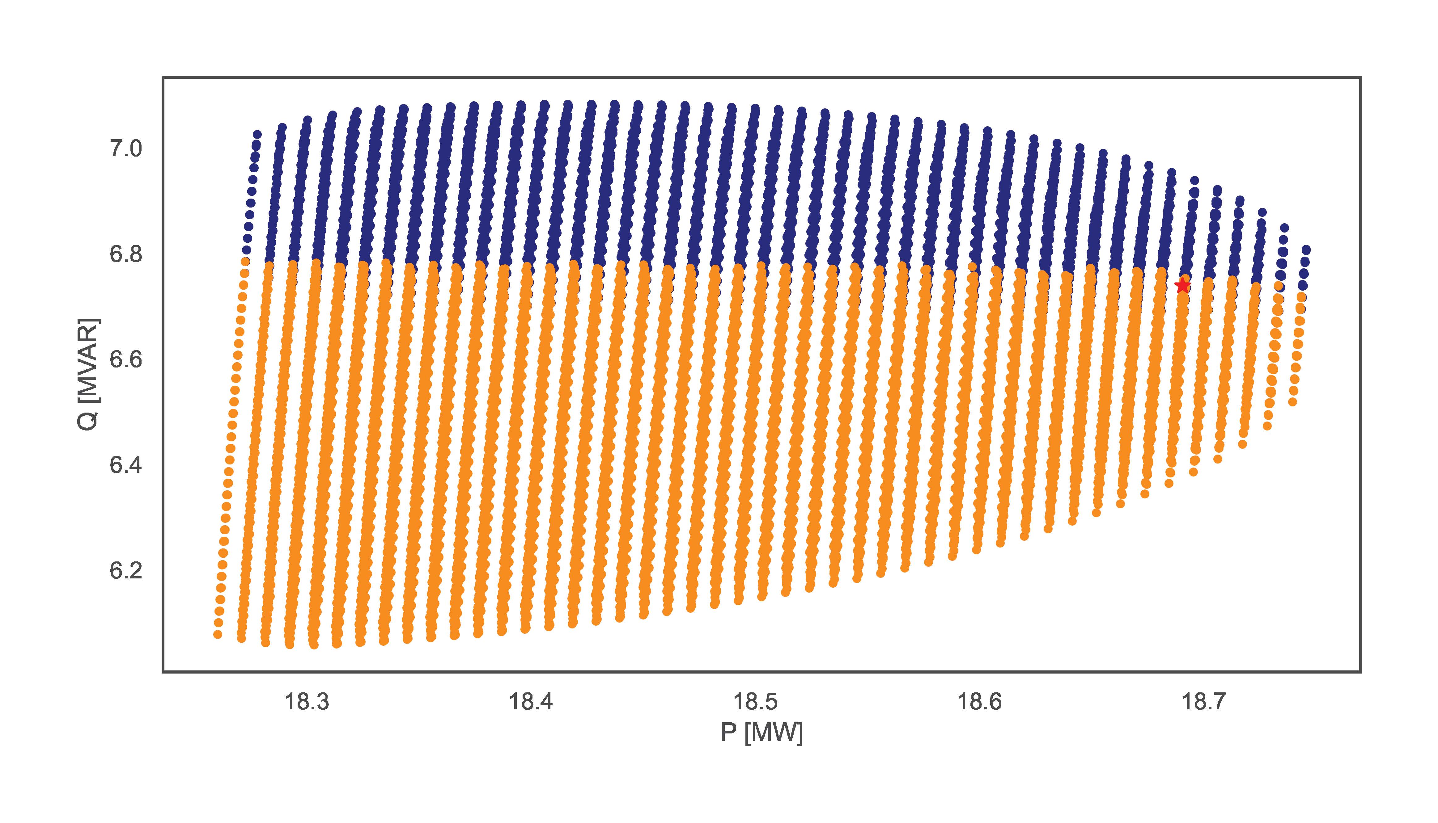
III.D) TensorConvolution+
This section illustrates examples using the TensorConvolution+ FA estimation functionality. The first examples, showcasing the different shapes of flexibility from FSPs use the lines:
TCP.tc_plus(net_name='MV Oberrhein0', fsp_load_indices=[1, 2, 3], dp=0.05, dq=0.1, fsp_dg_indices=[1, 2, 3])

TCP.tc_plus(net_name='MV Oberrhein0', fsp_load_indices=[1, 2], dp=0.05, dq=0.1, fsp_dg_indices=[1, 2], flex_shape='PQmax')
The examples vary in number of FSPs and shapes of flexibility offers. The example without the flex_shape input automatically obtains the value ‘Smax’. The figures bellow illustrate the resulting FA for each line respectively.
TensorConvolution+ can also simulate FAs with FSPs offering discrete setpoints of flexibility. For such scenarios, the input non_linear_fsps specifies which of the FSPs are non linear. The example line is:
TCP.tc_plus(net_name='CIGRE MV', fsp_load_indices=[3, 4, 5], dp=0.05, dq=0.1, fsp_dg_indices=[8], non_linear_fsps=[8])The resulting figure is:
III.E) TensorConvolution+ Merge
This section showcases the function merging FSPs using the TensorConvolution+ algorithm. For this functionality, the max_fsps input determines the maximum FSPs for which a network component can be sensitive before merging their flexibility. The example line is:
TCP.tc_plus_merge(net_name='MV Oberrhein0', fsp_load_indices=[1, 2, 3], dp=0.025, dq=0.05, fsp_dg_indices=[1, 2, 3], max_fsps=5)The resulting figure is:
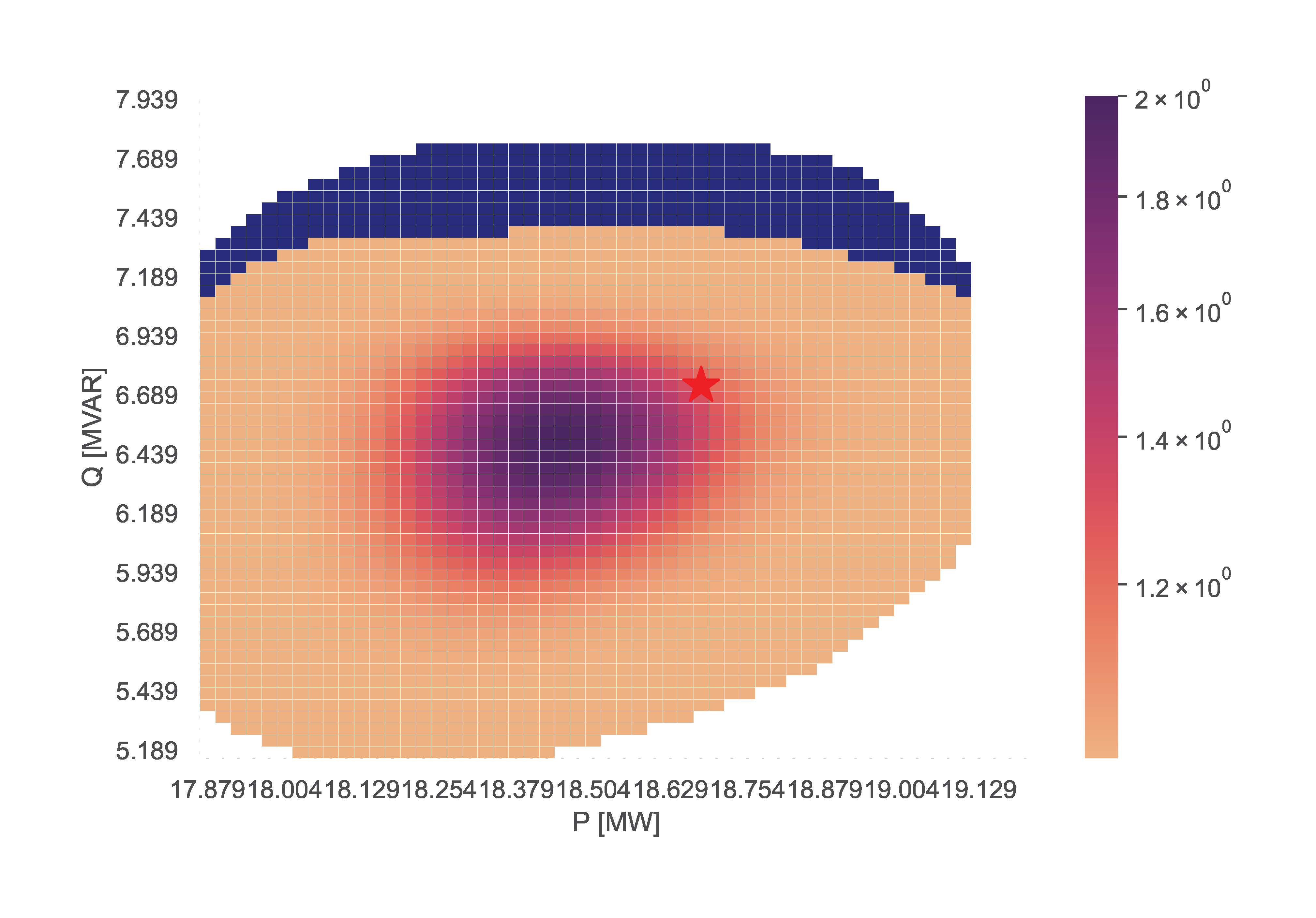
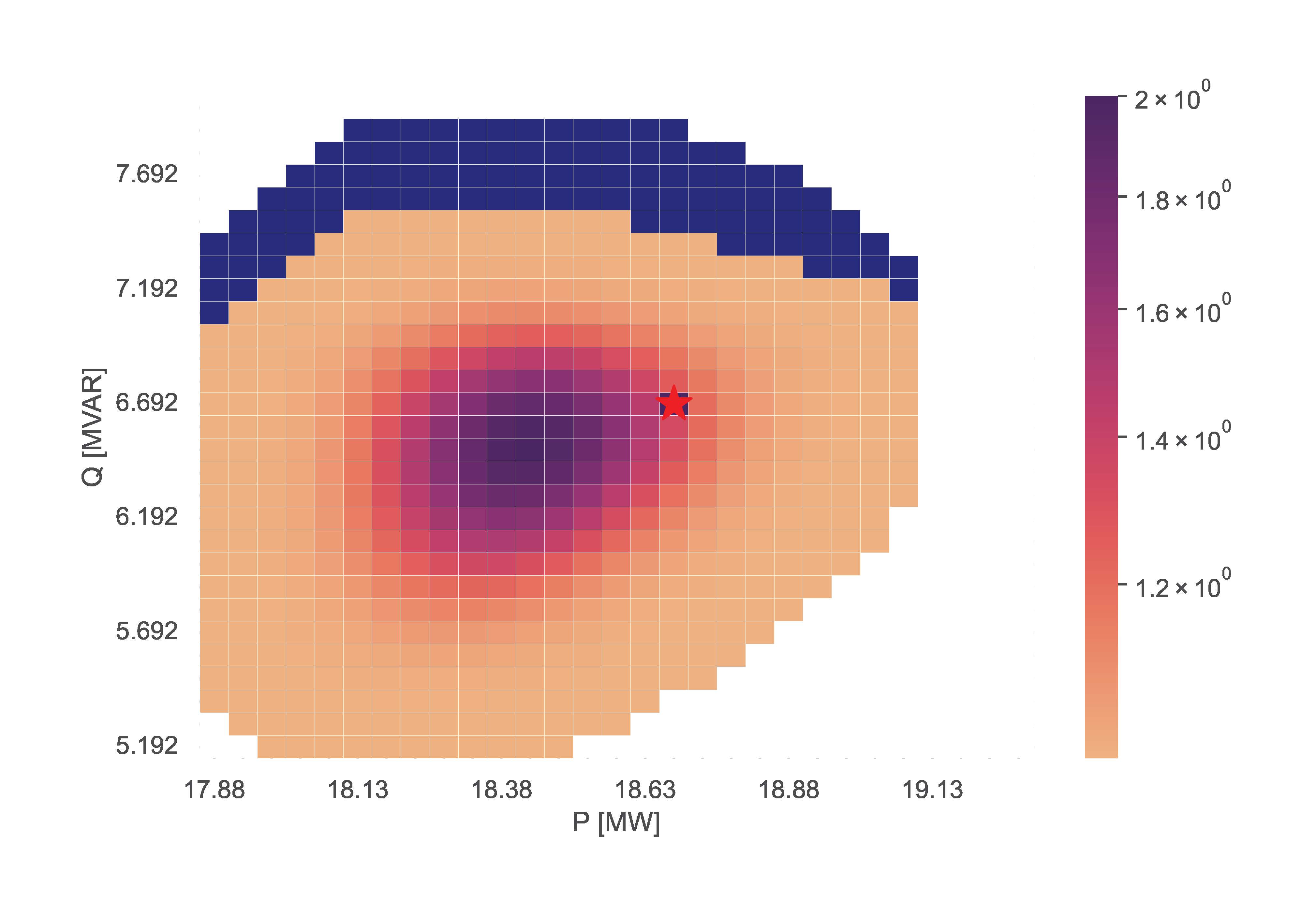
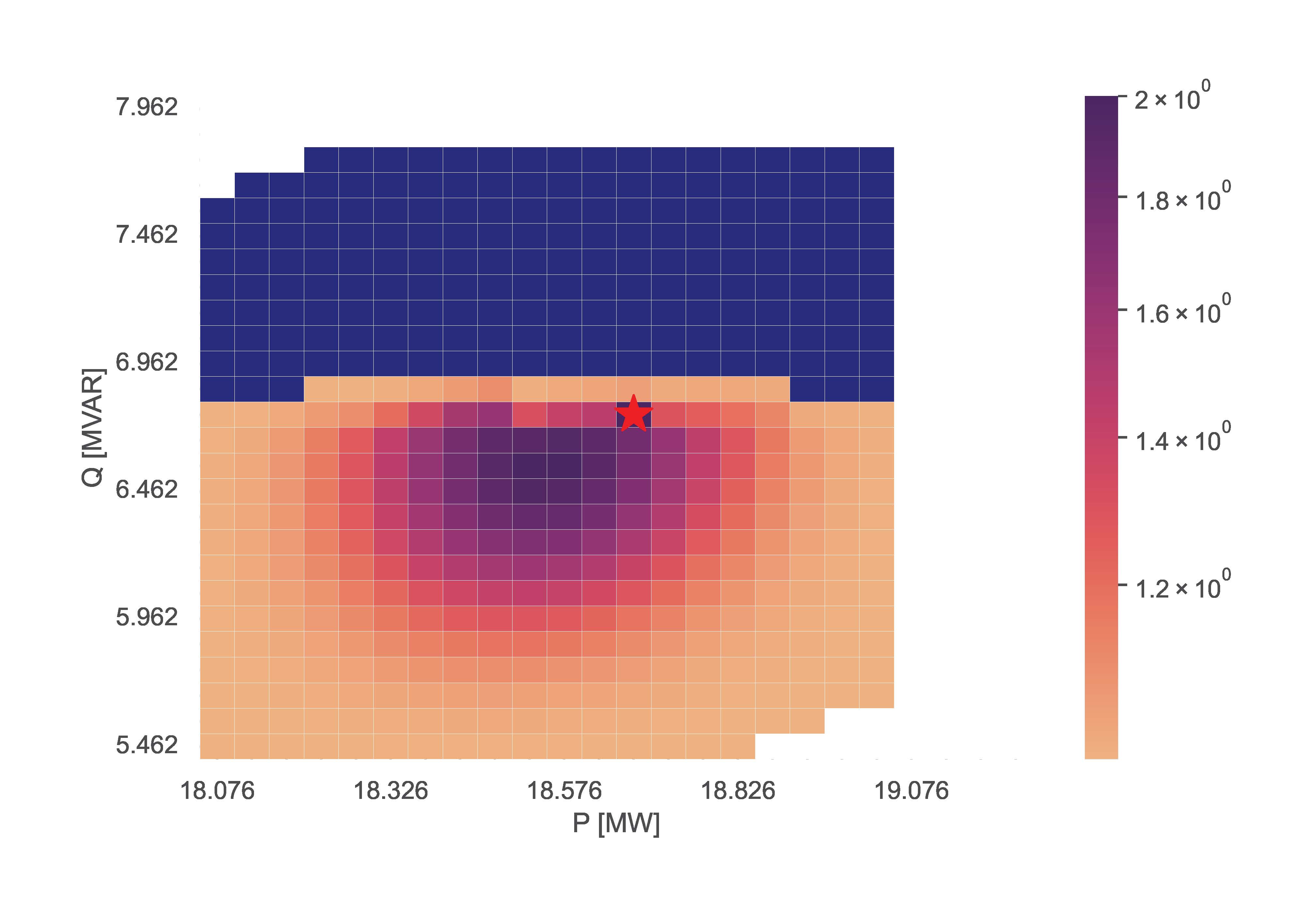
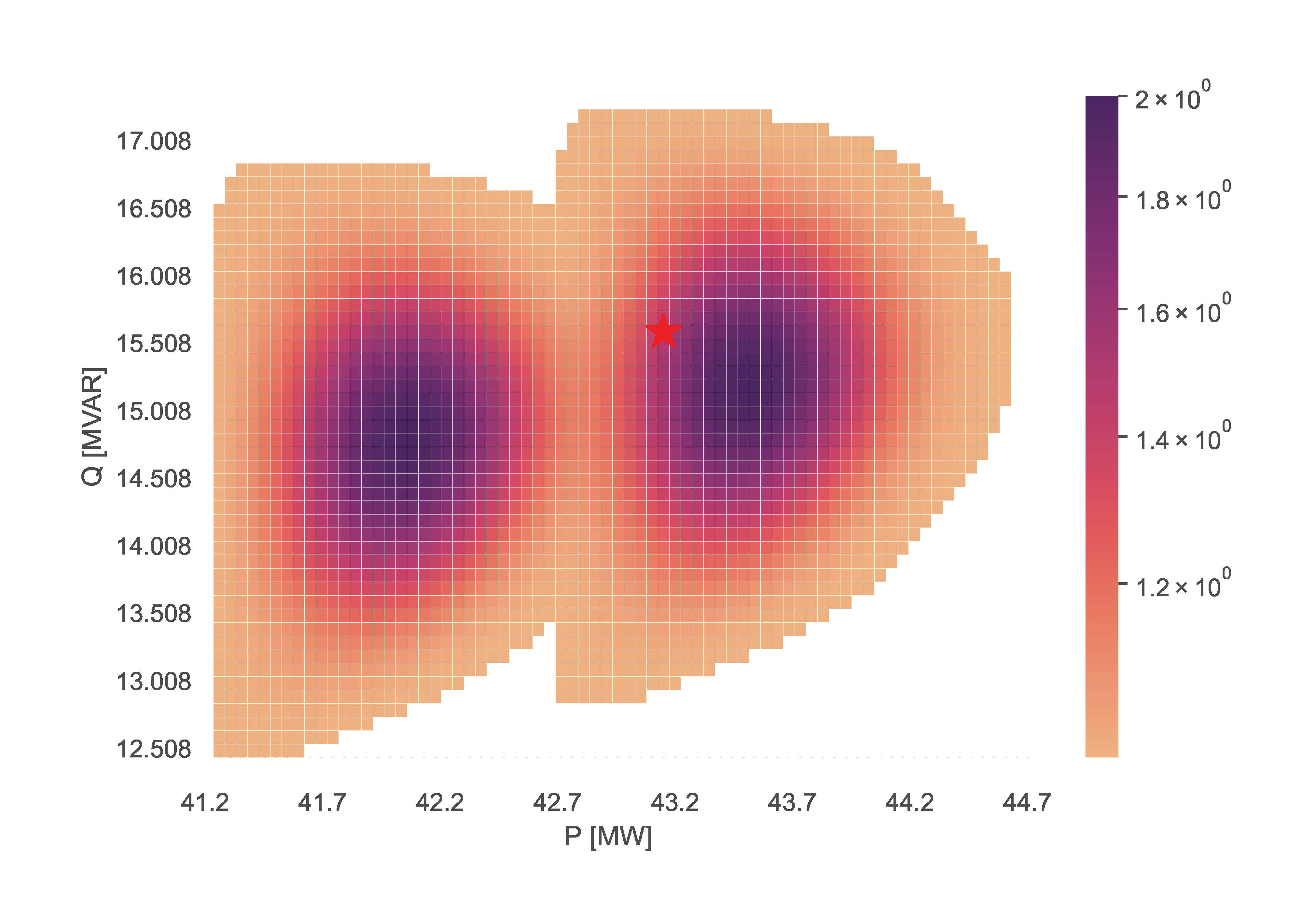
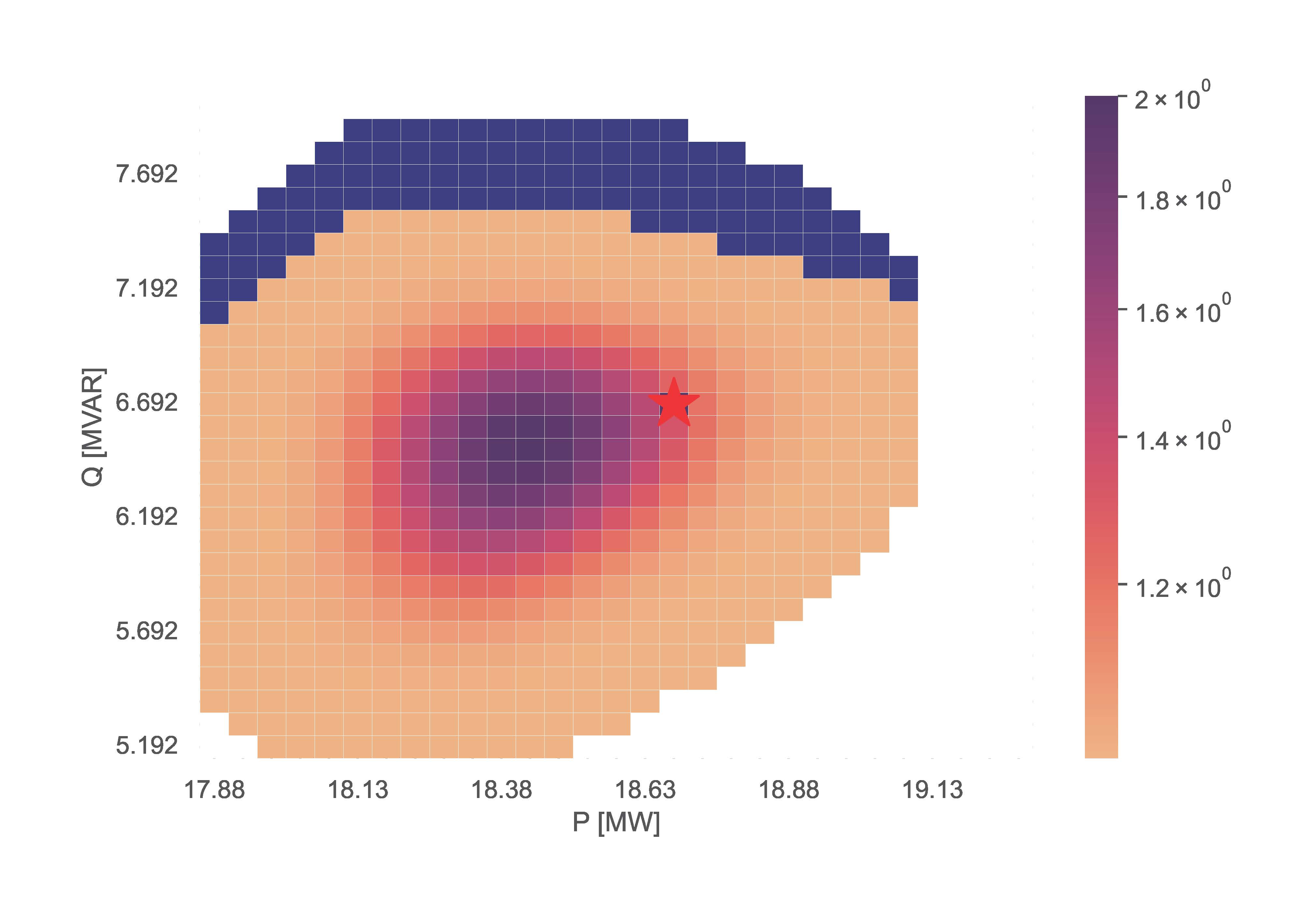
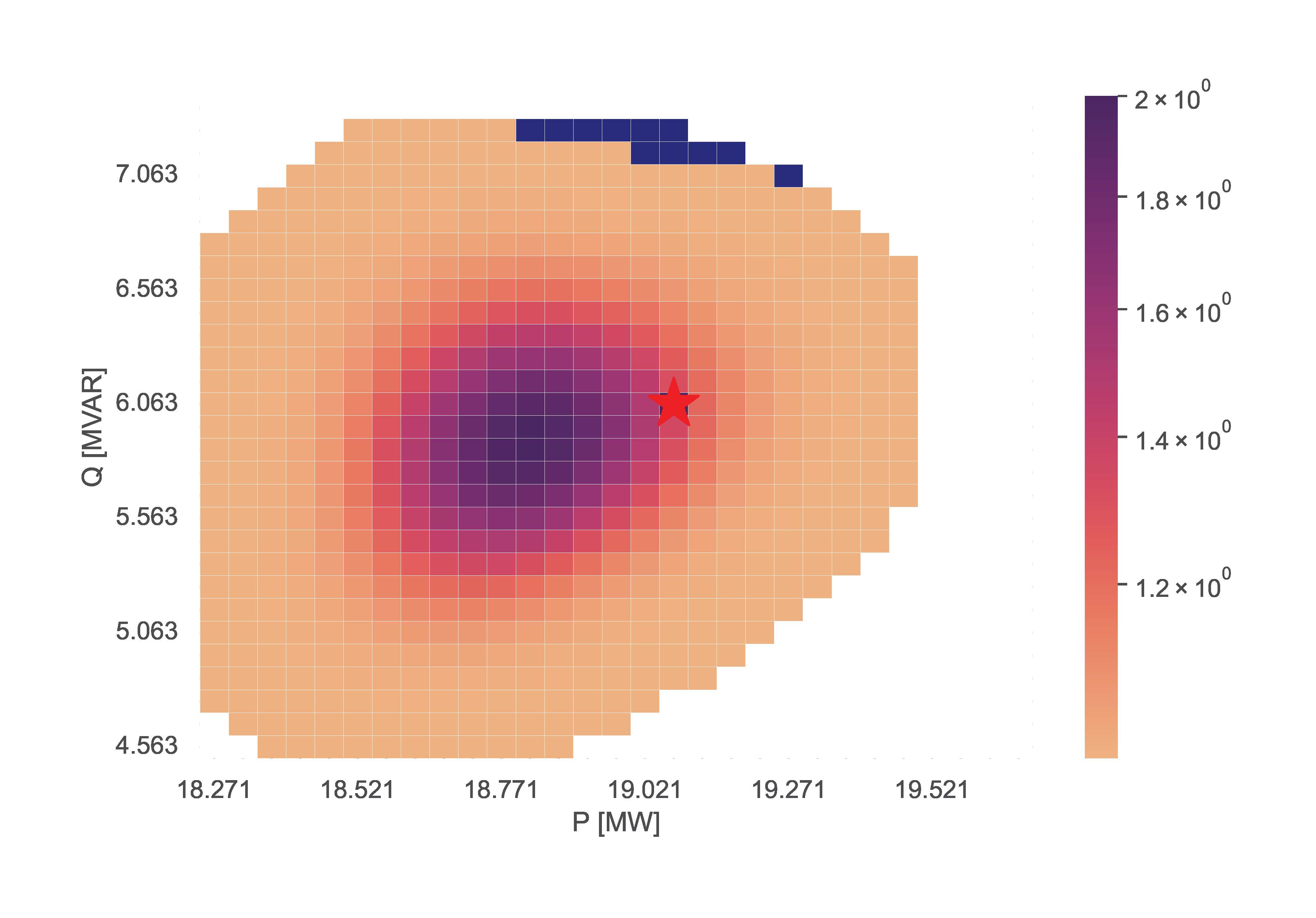
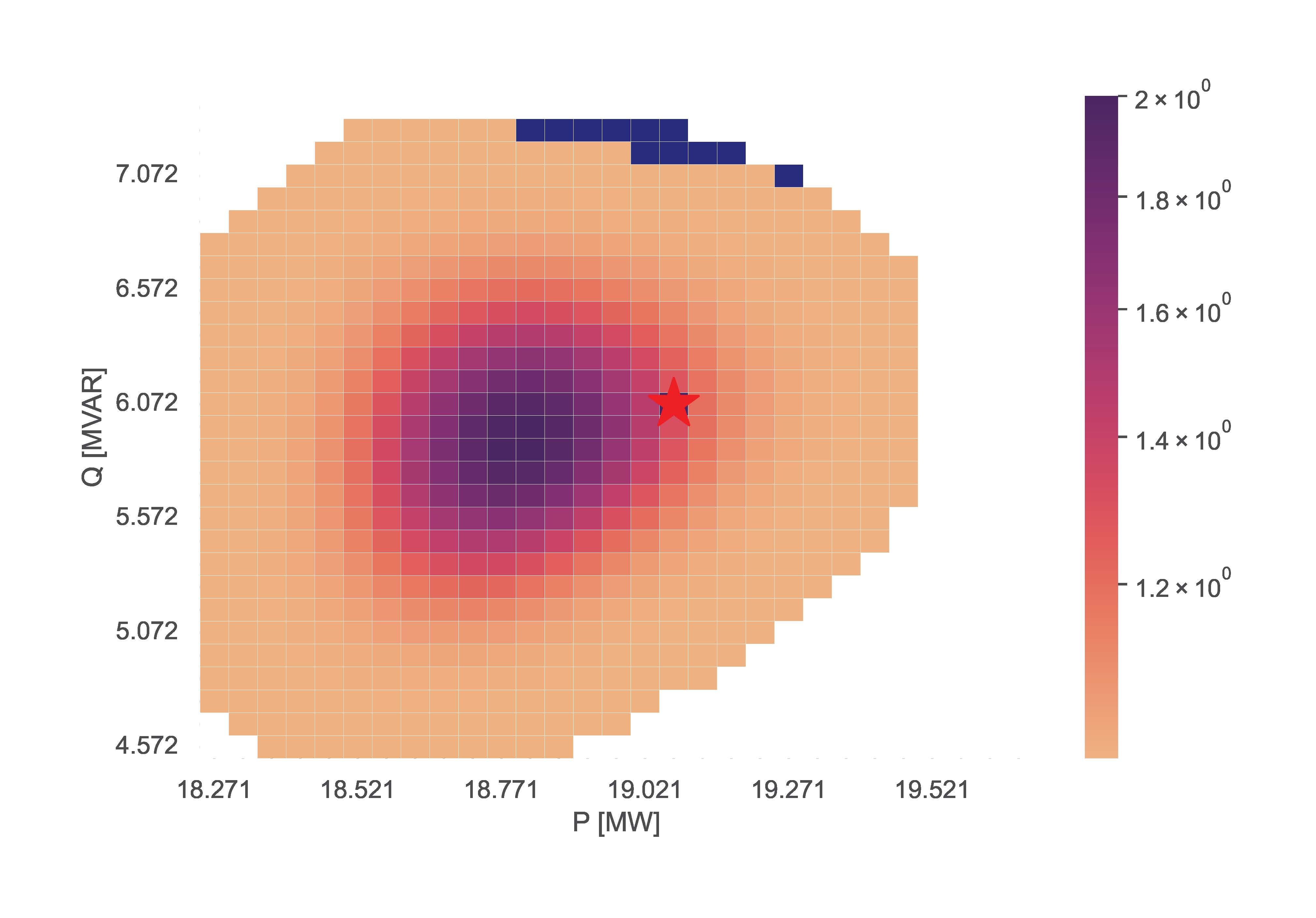
III.F) TensorConvolution+ Adapt
This section showcases the function storing information using the TensorConvolution+ algorithm, and then uses the stored information to adapt flexibility area for altered operating conditions.
# Define the consistent FSPs for the storing and adapting functions
fsp_load_indices = [1, 2, 3]
fsp_dg_indices = [1, 2, 3]

# Estimate the FA and store the relevant information for adaptation
TCP.tc_plus_save_tensors(net_name='MV Oberrhein0', fsp_load_indices=fsp_load_indices, dp=0.05, dq=0.1, fsp_dg_indices=fsp_dg_indices)

# Modify the network operating conditions
net, net_tmp = pn.mv_oberrhein(separation_by_sub=True)
net.load['sn_mva'] = list(net.load['p_mw'].pow(2).add(net.load['q_mvar'].pow(2)).pow(0.5))
net.load['scaling'] = [1 for i in range(len(net.load))]
net.sgen['scaling'] = [1 for i in range(len(net.sgen))]
net.switch['closed'] = [True for i in range(len(net.switch))]

net = fix_net(net) # This function is included in the appendix

rng = np.random.RandomState(212)

net, rng = rand_resample(net, fsp_load_indices, fsp_dg_indices, rng, 0.05, 0.01, 0.05, 0.01) # This function is also included in the appendix

# Adapt the FA using the locally stored information
TCP.tc_plus_adapt(net=net, fsp_load_indices=fsp_load_indices, fsp_dg_indices=fsp_dg_indices)

# Estimate the FA without adapting to compare with the above adapted result
TCP.tc_plus(net=net, fsp_load_indices=fsp_load_indices, fsp_dg_indices=fsp_dg_indices, dp=0.05, dq=0.1)
The resulting figures for the stored, adapted and validated flexibility areas are:
Release history Release notifications | RSS feed


Download files
Download the file for your platform. If you're not sure which to choose, learn more about installing packages.
Source Distribution
Built Distribution
Filter files by name, interpreter, ABI, and platform.
If you're not sure about the file name format, learn more about wheel file names.
Copy a direct link to the current filters
File details
Details for the file tensorconvolutionplus-0.1.1.tar.gz.
File metadata
- Download URL: tensorconvolutionplus-0.1.1.tar.gz
- Upload date:
- Size: 4.8 MB
- Tags: Source
- Uploaded using Trusted Publishing? No
- Uploaded via: twine/6.0.1 CPython/3.10.5
File hashes
| Algorithm | Hash digest | |
|---|---|---|
| SHA256 |
37fdc4baf9d814715cefde8b19ae3f2b9f9b72f366c51dc67e1f3f764a518d14
|
|
| MD5 |
86c4269115a22b29eaca501b3ec351ca
|
|
| BLAKE2b-256 |
71508103ef4dc08530b90ca4135ce13321babe0a47d820bbf7c99207dd8240c3
|
File details
Details for the file TensorConvolutionPlus-0.1.1-py3-none-any.whl.
File metadata
- Download URL: TensorConvolutionPlus-0.1.1-py3-none-any.whl
- Upload date:
- Size: 68.2 kB
- Tags: Python 3
- Uploaded using Trusted Publishing? No
- Uploaded via: twine/6.0.1 CPython/3.10.5
File hashes
| Algorithm | Hash digest | |
|---|---|---|
| SHA256 |
a4c56ef3c9b10d9c01de8b8de2d1a9065ee0e5eb0ada0e87d0c57e8f5f357ba6
|
|
| MD5 |
cd08396108cb80674e57e8fda321169a
|
|
| BLAKE2b-256 |
81920f632f4319da4a23eb6305b40bab39d5312ba164406ef70bbe3b7e8418c6
|


