
CRAMM





General-purpose hyperspectral mineral identification toolkit — built on the USGS MICA (Material Identification and Characterization Algorithm) decision-rule system. The classification core is sensor-agnostic: it works on any VNIR–SWIR reflectance cube given its band configuration (center wavelengths, FWHM, valid-band mask), because the bundled 1 nm rule-face reference spectra are resampled to the sensor's bands at runtime. EMIT L2A is simply the built-in data reader — one supported input type, not the defining one.
CRAMM extends MICA in three ways:
- An enhanced rule schema. CRAMM adds an optional secondary-feature
depth-ratio constraint (
max_depth_ratio_feat1_over_feat0) that rejects pixels whose secondary absorption is too deep relative to the primary 2.2 µm feature — suppressing white-mica false positives that pass the original five-layer MICA filtering. Nine bundled rules (muscovite, illite, kaolinite–muscovite mixtures) carry the new constraint; any custom rule can opt in. See Enhancements over USGS MICA. - Wavelength-arbitrated muscovite subtyping. MICA labels a pixel
"muscovite_lowAl / medAl / medhighAl / Fe-rich" by best fit alone; CRAMM
then re-arbitrates that attribution with the pixel's fitted 2.2 µm
absorption center against per-rule calibrated wavelength windows
(
absorption_center_range) — the spectroscopically meaningful axis along which these four subtypes are actually defined. See Enhancements over USGS MICA → Wavelength-based muscovite attribution. - From mineral detection to mineral composition. Beyond labeling
muscovite pixels, CRAMM fits the per-pixel 2.2 µm absorption-center
wavelength (
mus_center) — a quantitative composition proxy whose thermodynamic basis (Tschermak substitution vs. wv2200 on a GEMS/MINES23.1 reaction-path phase diagram) turns each fitted pixel into a calibrated constraint on muscovite chemistry and on its position in the T–log(aK⁺/aH⁺) plane. See Application: reading muscovite composition from mus_center.
Everything is pure Python and GUI-free. Cross-platform: Windows / Linux / macOS · Python 3.9 – 3.13
Highlights
- Enhanced MICA pipeline — continuum removal → closed-form 2×2 least squares → fit (r²) & absorption depth → five-layer constraint filtering + the CRAMM depth-ratio constraint, driven by a JSON rule library (77 rules covering clay, sulfate, carbonate, mica, chlorite, amphibole, iron oxide, snow/ice and their mixtures).
- Quantitative muscovite mapping — per-pixel 2.2 µm absorption-center wavelength as a dedicated thematic map and float array; the same center also re-arbitrates the lowAl / medAl / medhighAl / Fe-rich attribution against calibrated wavelength windows, with a phase-diagram interpretation framework.
- Quantitative chlorite mapping — per-pixel 2250 nm absorption-center
wavelength (
chl_center) for pixels won by the four pure-chlorite rules, as a fourth thematic map and float array; a continuous Fe-content proxy anchored by the chl13 calibration (LOO 1.0 nm). The same center also re-arbitrates the lowFe / clinochlore / Fe-rich / thuringite attribution against calibrated wavelength windows that tile the 2.245–2.266 µm range without overlap, so every in-range center arbitrates to exactly one subtype. - Quantitative carbonate mapping — per-pixel 2330 nm absorption-center
wavelength (
cal_center) for pixels won by the six carbonate rules, as a fifth thematic map and float array; band position tracks the seven-anchor C–O sequence (magnesite 2311 nm → rhodochrosite ~2369 nm), making species the rule library cannot tell apart (aragonite, magnesite — silently classified as dolomite) visible in the continuous layer. The same center also arbitrates the dolomite ↔ calcite attribution within each abundance tier (v1.5.0): the abundant pair and the plain pair compete separately against disjoint windows, a 6 nm dead zone shelters siderite-ish centers, and the abundance axis never crosses. - Whole-scene and single-spectrum modes — batch-classify an entire scene to GeoTIFF, or identify one spectrum (GUI point-click, field spectrometer) with Top-N ranking and a PDF diagnostic report.
- Sensor-agnostic core — everything downstream of data loading consumes a
generic
(spectrum, wavelengths, FWHM, valid bands)contract. The bundled reader covers EMIT L2A NetCDF; any other sensor (airborne or spaceborne) plugs in through the same seven-tuple — no rule or code changes needed. - Fast — reference-side constants are precompiled once per band configuration (two-level cache; ~16× speedup on repeated single-spectrum calls), and scene classification parallelizes across rules with worker processes.
- Bit-exact discipline — serial and parallel paths produce identical bytes; every change is guarded by a dual-path golden regression suite.
- Self-contained — the rule library (
cramm/data/temp_rf_notfeatures_renamed.json), the 1 nm rule-face spectra bundle (cramm/data/rf77_splib07_1nm.npz), and the mineral color table are bundled inside the wheel.
How it works
Hyperspectral reflectance cube (any VNIR–SWIR sensor)
      │  built-in: load_emit (EMIT L2A NetCDF, bad-band removal)
      │  or your own loader → (spectrum, wl, w, bp, chanels)
      ▼
Reference resampling ── 1nm rule-face spectra ──► sensor wavelengths/FWHM
      │                                        (Gaussian kernel, cached)
      ▼
Per-rule evaluation (77 rules, parallel across rules)
      │  diagnostic features: continuum removal → 2×2 LSQ → r² / depth
      │  not-absorption / not-related features: exclusion filters
      │  continuum & depth-ratio constraints
      ▼
Best-match selection (argmax weighted fit)  +  muscovite 2.2 µm center fit
      │                                   +  chlorite 2250 nm center fit
      │                                   +  carbonate 2330 nm center fit
      ▼
Wavelength-arbitrated subtyping (muscovite / chlorite / carbonate families)
      │  *_center vs. per-rule absorption_center_range windows
      ▼
Mineral map · color-enhanced map · muscovite map · chlorite map · carbonate map
(+ raw float arrays: mus_center / chl_center / cal_center / fd)
Installation
pip install cramm            # core features (PyPI wheels on all three platforms)
pip install cramm[tiff]      # + GeoTIFF output (GDAL; PyPI wheels are Windows-only)
pip install cramm[pdf]       # + single-spectrum feature PDF diagnostics
pip install cramm[all]       # everything
GDAL on Linux/macOS: PyPI ships GDAL wheels for Windows only. Install a system libgdal first (conda-forge recommended), then install without deps:
conda install -c conda-forge gdal
pip install cramm --no-deps        # or: pip install cramm[pdf]
Without GDAL, only write_tiff (GeoTIFF output) is unavailable — all
classification and analysis functions work (lazy import).
From source (sdist / checkout):
pip install . # add [all] for the optional extras
Quick start
Command line
The CLI uses the built-in EMIT L2A reader; for other sensors, use the Python API (below) with your own loader.
cramm -i EMIT_L2A_RFL_001_xxx.nc -o output [-n scene] [-w 4] [--raw]
| Flag | Default | Meaning |
|---|---|---|
-i, --input |
(required) | Path to the EMIT L2A NetCDF file |
-o, --output |
. |
Output directory |
-n, --name |
input filename | Output filename prefix |
-w, --workers |
min(cpu, 8) |
Parallel worker processes (1 = serial) |
--raw |
off | Also save mus_center + chl_center + fd float arrays as .npz |
Output files (written to <output>/<name>*):
| File | Content |
|---|---|
<name>_mapping_orth.tiff |
Mineral map (orthorectified, rule-library colors) |
<name>_color_enhanced_orth.tiff |
Color-enhanced mineral map |
<name>_mus_orth.tiff |
Muscovite 2.2 µm absorption-center thematic map |
<name>_chl_orth.tiff |
Chlorite 2250 nm absorption-center thematic map |
<name>_cal_orth.tiff |
Carbonate 2330 nm absorption-center thematic map |
<name>_raw.npz |
(only with --raw) mus_center + chl_center + cal_center [μm] + fd (fit×depth), float [r, c] |
Python API
from cramm import MicaEngine

engine = MicaEngine()                                    # all resources bundled
spectrum, lon, lat, w, bp, wl, chanels = engine.load_emit("EMIT_xxx.nc")

# --- whole scene → GeoTIFF -------------------------------------------------
orth, color, mus, chl, cal = engine.spectrum_analysis(spectrum, wl, w, bp, chanels,
                                                      n_workers=4)
engine.write_tiff("output/scene", lon, lat, orth, color, mus, chl, cal)

# --- single spectrum (one pixel, field spectrometer, ...) ------------------
pixel = spectrum[100, 200, :]                            # full-band [285] or selected [len(chanels)]
results = engine.classify_spectrum(pixel, wl, w, bp, chanels,
                                   top_n=5, pdf_path="diag.pdf")
for r in results:
    print(f"{r['name']:50s} fit={r['fit']:.4f}  fd={r['fd']:.4f}")
Other sensors (non-EMIT data)
load_emit is only a convenience reader. For any other sensor, load the cube
yourself and pass the same band-configuration contract — references are
resampled to your wavelengths/FWHM automatically:
from cramm import MicaEngine
import numpy as np

engine = MicaEngine()
spectrum = my_loader("scene.dat")          # [rows, cols, bands] reflectance
w  = np.array([...])                       # band center wavelengths [µm]
bp = np.array([...])                       # band FWHM [µm]
chanels = np.arange(len(w))                # valid bands (drop bad-band indices)
wl = w[chanels]

orth, color, mus, chl = engine.spectrum_analysis(spectrum, wl, w, bp, chanels,
                                                 n_workers=4)
Only the map rendering (write_tiff) needs geolocation (lon/lat grids);
classification itself is purely spectral and location-free.
classify_spectrum returns a list of {"name", "fit", "fd"} dicts sorted by
descending fit (empty list when nothing passes the filters). With
pdf_path= it also writes a multi-page PDF: one page per Top-N mineral with
continuum-removed feature overlays and constraint annotations (requires the
[pdf] extra).
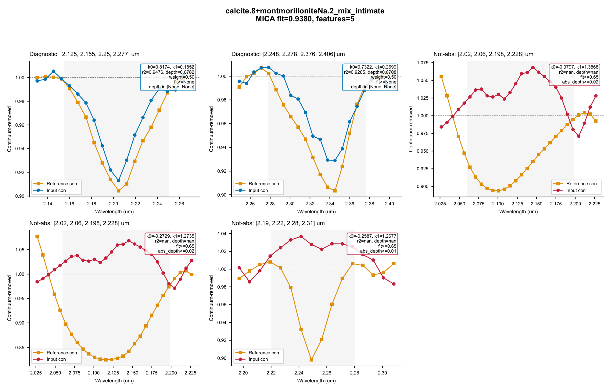
Each PDF page dissects one candidate rule — every diagnostic / not-absorption / not-relative feature with its continuum endpoints, the reference continuum-removed profile (squares) against the input (circles), and the full constraint audit (k0/k1, r², raw depth, weights, thresholds):
More scenarios — float (raw=True) output, custom rule libraries, the
invalidate_caches() contract, component-level calls — in
example_usage.py: python example_usage.py pixel.
API overview
MicaEngine method |
Purpose |
|---|---|
load_emit(path) |
(EMIT-specific convenience reader) Read EMIT L2A NetCDF → (spectrum, lon, lat, w, bp, wl, chanels); float32 cube, bad bands removed, fill values zeroed. Not needed for other sensors — supply the same tuple yourself |
spectrum_analysis(spectrum, wl, w, bp, chanels, ...) |
Classify a whole scene → 4 uint8 RGB images; raw=True adds mus_center + chl_center + fd float arrays. Supports progress_callback, log_callback, cancel_flag, n_workers |
classify_spectrum(spectrum, wl, w, bp, chanels, top_n=10, pdf_path=None) |
Identify one spectrum → Top-N [{"name", "fit", "fd"}] |
write_tiff(prefix, lon, lat, orth, color, mus, chl=None) |
Orthorectify (pyresample) and write the GeoTIFFs; chl is optional (omit for legacy 3-file output); requires GDAL |
get_resample(w, bp) |
All reference spectra resampled to the sensor bands {rule_name: spectrum} (cached; keys are rule-name strings — the sole link to the reference library after the v1.4.0 id purge) |
invalidate_caches() |
Required after mutating engine.rf in place — see below |
Custom rule libraries
engine = MicaEngine(rf_path="my_rules.json")          # at construction
# — or mutate in place —
engine.rf["my_mineral"] = {...}
engine.invalidate_caches()                            # mandatory!
The compiled-rule cache is keyed on band configuration only, not on rule
content. If you modify engine.rf after any classification call, you must call
invalidate_caches() (or build a new engine) — otherwise results silently use
the old reference-side constants.
Schema note (v1.4.0+): the rule library is id-free. Every
reference.reflectance_record (and every not_(abs/rel)_features[*].reflectance_record)
must be a rule-name string drawn from the top-level rf keys; the loader
verifies this contract at construction and rejects any non-string or
unresolved reference. Custom rules cloning an existing rule set
reference.reflectance_record to the source rule's name — the spectrum is
then inherited from the 1 nm bundle row indexed by that name (the clone
itself has no row in the bundle).
Cache contract (v1.4.1+): reassigning engine.rf to a different dict
object (engine.rf = new_dict) is detected automatically via an id()
snapshot and the cache is dropped; in-place value mutation
(engine.rf["x"] = ...) and in-place key addition (engine.rf["new"] = ...)
are not detected — the former silently keeps stale results, the latter
raises KeyError from the compiled-rules cache (a deliberate stale-trap).
Both require an explicit invalidate_caches() call.
1 nm rule-face track
The classifier runs the 1 nm rule-face track exclusively — reference
spectra baked onto a shared 1 nm master grid (350–2500 nm) in
cramm/data/rf77_splib07_1nm.npz (77 rule-face rows); no splib06b / specpr / external
library is needed at runtime. The rule library
cramm/data/temp_rf_notfeatures_renamed.json carries the same 77 rules as the
historical USGS .mcf v6a. As of v1.4.0 the rule library is id-free:
every reference.reflectance_record (and every
not_(abs/rel)_features reflectance_record) is a rule-name string drawn
from rf.keys() — the rule name is the sole link between the rule library
and the 1 nm bundle. Of the 19 rules whose spectra were historically
engine-synthesized from multi-endmember recipes (mixtures), 14 are
bit-identical to the legacy library (12 engine-synthesized + 2
weight-1.0 aliases of measured GDS212/213 records) and 5 are weight-1.0 aliases
of splib07's AMX calculated-mixture records (mix_7821/7715/7711/7745/7737);
all 19 now ship as pre-baked rows in the npz bundle, so runtime
synthesis is no longer needed and the mixtures top-level key has been
removed from the JSON.
The reference_track parameter on MicaEngine / MicaClassifier.from_paths
is kept for API compatibility but ignored; passing anything other than
None / "1nm" raises ValueError.
Enhancements over USGS MICA
CRAMM extends the original USGS MICA decision rules with an optional per-rule
secondary-feature depth-ratio constraint,
max_depth_ratio_feat1_over_feat0:
After the standard MICA filtering, a rule carrying this key rejects any pixel where
raw_depth(feat1) / raw_depth(feat0) ≥ threshold, using the unweighted feature depths(1 − min(continuum-removed)) × k0. Pixels with an invalid primary feature (NaN depth) are conservatively kept.
For white micas the primary 2.2 µm Al-OH absorption (feat0) must dominate the secondary ~2.35 µm feature (feat1); a secondary absorption that is too deep relative to the primary indicates look-alike minerals rather than muscovite / illite. Nine bundled rules use this constraint:
| Threshold | Rules |
|---|---|
0.6 |
muscovite_lowAl, muscovite_medAl, muscovite_medhighAl, muscovite_Fe-rich, illite_imt1, illite_gds4 |
0.4 |
kaolinite.5+muscoviteMedAl.5, kaolinite.5+muscoviteMedhighAl.5, kaolinite+muscovite_mix_intimate |
The constraint is part of the rule schema — custom rule libraries can set
"max_depth_ratio_feat1_over_feat0": <float> on any rule with ≥2 diagnostic
features; omitting the key disables it (original MICA behavior).
Wavelength-based absorption-center attribution
CRAMM also adds an optional per-feature absorption-center window,
absorption_center_range on a rule's first diagnostic feature. After the
best-match selection, pixels attributed to a rule carrying this field are
re-arbitrated by their fitted absorption center (mus_center at 2.2 µm for
the white-mica family, chl_center at 2250 nm for the chlorite family,
cal_center at 2330 nm for the carbonate family):
If the center falls inside exactly one rule's
[lo, hi)window, differs from the current match, and that rule itself accepted the pixel, the pixel is reassigned to the matching rule (fit/depth/index follow, and the center is refitted once with the new rule's endpoints). An invalid center, a center outside every window, or a center inside several overlapping windows keeps the original match (conservative).
The four bundled pure-muscovite rules carry calibrated windows (anchored on
each reference spectrum's measured wv2200): medhighAl [2.195, 2.200),
medAl [2.200, 2.206), lowAl [2.206, 2.210), Fe-rich [2.210, 2.220) —
the four windows tile the 2.195–2.220 µm range without overlap, so every
valid center arbitrates to exactly one subtype. The four bundled
pure-chlorite rules likewise carry tiling windows — lowFe
[2.245, 2.248), clinochlore [2.248, 2.252), Fe-rich [2.252, 2.256),
thuringite [2.256, 2.266) — covering the 2.245–2.266 µm range without
overlap, so every in-range chl_center also arbitrates deterministically
to exactly one subtype (see Application: reading chlorite Fe content
from chl_center). The four calcite/dolomite rules form two abundance
tiers — calcite_abundant vs dolomite_abundant, and calcite vs dolomite —
which since v1.5.0 are arbitrated in two separate per-tier calls.
Within each tier the windows are disjoint (dolomite [2.308, 2.328) vs
calcite [2.334, 2.350)), so an in-window center arbitrates
deterministically to the other mineral of the pair; the two tiers never
mix, locking the abundance axis (abundant vs plain) structurally. A 6 nm
dead zone [2.328, 2.334) between the windows conservatively keeps
siderite-ish centers (~2327 nm anchor) on their argmax winner. On the
EMIT test scene this flipped 1599 pixels (0.10 % of the scene)
calcite→dolomite, with zero reverse flips and zero abundant-tier flips
(pinned by a dedicated unit test; see Application: reading carbonate
species from cal_center).
This is a scene-classification feature; single-spectrum Top-N ranking is
unaffected. Each arbitration call locks its group to one mineral family
(MUSCOVITE_MINERALS / CHLORITE_MINERALS — and for carbonates, one
abundance tier per call: CARBONATE_ABUNDANT_MINERALS or
CARBONATE_PLAIN_MINERALS — ∩ windowed rules), so cross-family and
cross-tier flips are structurally impossible
(pinned by a dedicated unit test). Custom rule libraries opt in per
family: append the new rule to the corresponding family list AND give it
the field; rules without it are never reassigned.
Seven white-mica-group and chlorite rules carry parsed structural formulas
of their reference spectra as bundled metadata:
reference.structural_formula with structural_formula_tier (A =
wet-chemistry Fe³⁺/Fe²⁺ split, B = total-Fe convention). White micas
(O=11 anhydrous basis, from the 14-sample white-mica
composition–band-position calibration set): muscovite_medhighAl (GDS113),
muscovite_Fe-rich (GDS116), illite_gds4 (GDS4) and illite_imt1 (IMt-1) —
of the four arbitration windows above, medhighAl and Fe-rich are thereby
anchored to measured chemistry; medAl (CU91-250A) and lowAl (CU93-1) have
no published full analysis. Chlorites (O₁₀(OH)₈ basis, from the chl13
calibration set): chlorite_lowFe (SMR-13), clinochlore (GDS158) and
clinochlore_Fe (SC-CCa-1; chemistry from the Bartel XRF of the same CMS
CCa-1 specimen) — the full lowFe→Fe-rich gradient is chemistry-anchored.
The metadata is informational only and never enters the classification
math.
Application: reading muscovite composition from mus_center
The muscovite thematic map's per-pixel mus_center (2.2 µm Al-OH absorption
position) is a quantitative proxy for muscovite chemistry. The phase diagram
below — a GEMS/MINES23.1 titration reaction-path model of the
K₂O–Al₂O₃–SiO₂–H₂O–HCl–FeO–MgO system — overlays the Tschermak substitution
degree X_Ts = X(Fe-Celadonite)+X(Celadonite) in the muscovite stability field
with the corresponding wv2200 position (USGS conversion chain:
X_Ts → Al₂O₃ wt% → λ = −3.1·Al₂O₃ + 2308):
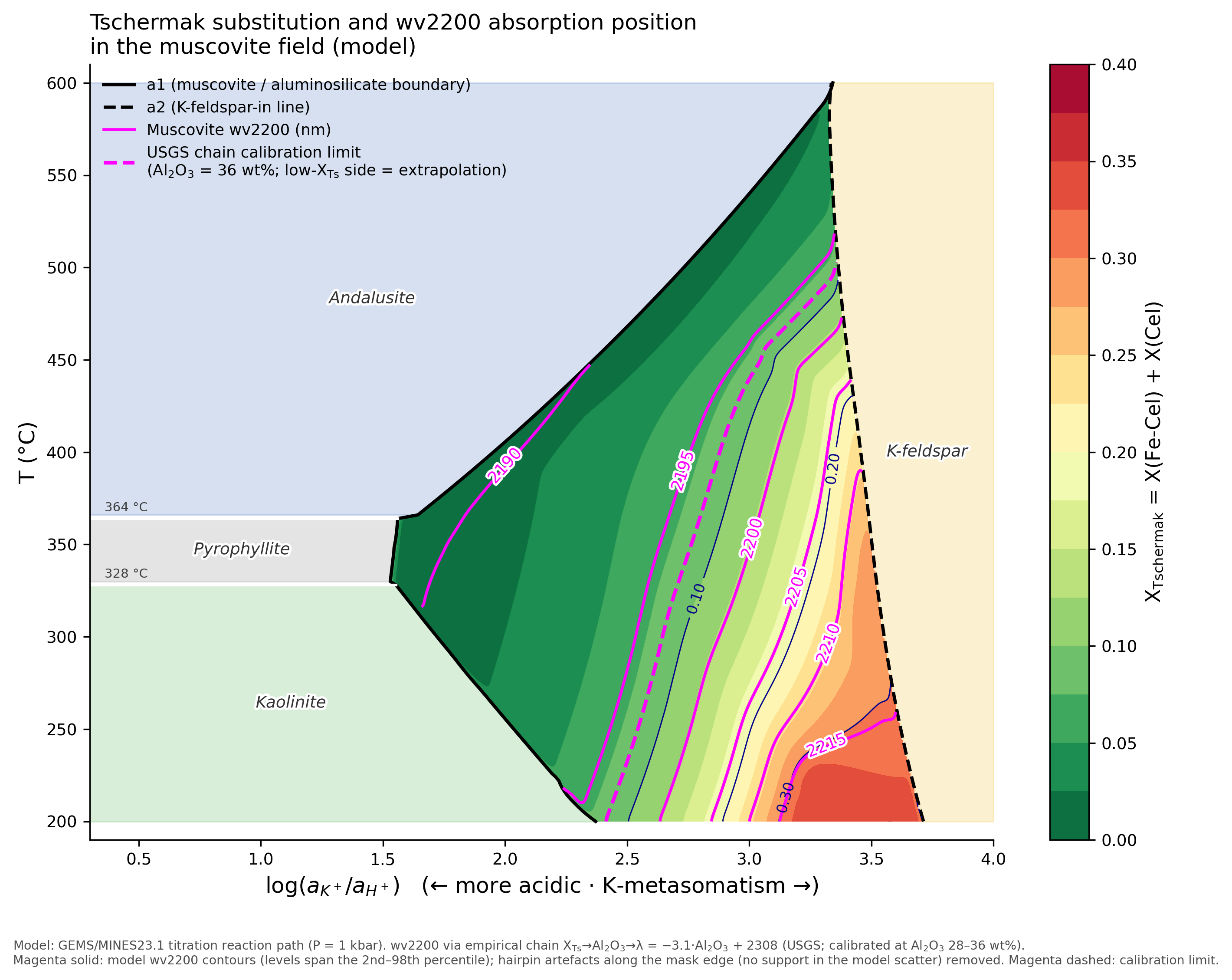
X_Ts rises from ~0 on the high-T / low-K⁺ side to 0.35+ on the low-T / high-K⁺
side. The wv2200 contours (magenta, 2190→2215 nm) are derived by chaining the
empirical wavelength–composition calibration through the modelled X_Ts field,
so they track the X_Ts contours (dark blue) by construction. Each mus_center
value fitted from an image pixel therefore selects one isopleth on this
diagram: muscovite composition (X_Ts) is read directly, while in the
T–log(aK⁺/aH⁺) plane the value defines a one-dimensional constraint locus,
not a unique point. Pinning down both formation temperature and fluid K⁺/H⁺
requires a second independent constraint — e.g. the chl_center of a
coexisting chlorite read on the companion diagram, under a same-pressure,
same-fluid equilibrium assumption. The diagram is an interpretive framework
for the product, not a ground-validated inversion.
Application: reading chlorite Fe content from chl_center
The chlorite thematic map's per-pixel chl_center (2250 nm Fe–OH absorption
position) is a continuous composition proxy: across the chl13 calibration
set (13 samples spanning xFe 0.014–0.553) the closed-form model
pos2250 = 2218.8·xAl + 2279.6·xFe + 2249.7·xMg reproduces band positions
with LOO-RMSE 1.0 nm — at the repeat-measurement noise floor — and the
calibration is immune to the Fe²⁺/Fe³⁺ reporting convention (closure
normalization cancels it exactly). Like the muscovite subtypes, the four
chlorite rules carry tiling windows without overlap: lowFe [2.245, 2.248),
clinochlore [2.248, 2.252), Fe-rich [2.252, 2.256), thuringite
[2.256, 2.266) µm. Every in-range chl_center
therefore hits exactly one window and arbitrates deterministically to one
subtype, with the center refitted once against the target rule's
endpoints; only an invalid center or one outside every window keeps the
argmax attribution. Practical limits from the
calibration: quantitative inversion needs chlorite ≳50 % of the pixel and a
comparable sample preparation; the 2350 nm Mg–OH band (cross-instrument
anchor, bias ≈0.2 nm) is reserved for pure-mineral checks.
Application: reading carbonate species from cal_center
The carbonate thematic map's per-pixel cal_center (2330 nm C–O absorption
position) discriminates carbonate species along the seven-anchor band
sequence: magnesite 2311 nm < aragonite 2315 nm < Fe-dolomite 2319 nm <
dolomite 2321 nm < siderite ~2327 nm < calcite 2339 nm < rhodochrosite
~2369 nm (Fe²⁺ substitution blue-shifts the band by ~2 nm; Mn²⁺ red-shifts
it). The bundled rule library covers only three of these anchors — calcite
(WS272), dolomite (HS102.3B) and a manganoan siderite (HS271, inherited from
USGS MICA as carbonate_Fe_bearing) — so aragonite and magnesite pixels are
silently classified as dolomite by best fit. cal_center makes them
visible: a "dolomite" pixel whose center sits at 2311–2316 nm is a
magnesite/aragonite suspect, and the continuous layer likewise exposes
Fe-bearing dolomite (≤2319 nm) inside the dolomite class. Since v1.5.0 the
wavelength arbitration does reassign carbonate pixels — but only within an
abundance tier: a "calcite" pixel whose center falls in the dolomite window
[2.308, 2.328) flips to dolomite (and vice versa within the pair), while
abundant and plain never cross, and the 6 nm dead zone [2.328, 2.334)
keeps siderite-ish centers on their argmax winner. On the EMIT test scene
this produced 1599 calcite→dolomite flips (0.10 % of the scene; flipped
centers 2314–2328 nm, i.e. Fe-bearing-dolomite band positions), zero
reverse flips and zero abundant-tier flips. The map bins the
post-arbitration centers at 5 nm steps over [2.308, 2.358) µm, shorter
wavelength = earlier anchor in the sequence above.
Performance notes
- Precompiled rules: continuum endpoints, band indices, the reference-side
normal-equation constant
Band depth factors are computed once per(wavelengths, FWHM, valid-band)configuration and reused across all pixels and calls. - Parallelism: scene classification fans out across the 77 rules with
multiprocessing(spawn context). The per-pixel normal-equation solve (k0/k1) is a BLAS-freenp.einsum, so results are independent of the pixel-row count and the BLAS thread pool — the parallel path is bit-identical to the serial one structurally, not by BLAS-configuration luck (worker BLAS pinning to a single thread is retained as defense in depth). - Typical runtime: a full scene (e.g. an EMIT granule, ≈1280×1242 pixels) classifies in about a minute with a few workers on a desktop; a warm single-spectrum call is ≈10 ms.
Testing
python tests/test_core.py              # 21 API contract / behavior tests
                                       # (integration section auto-skips without the test scene)
python tests/test_custom_rules.py      # custom rule-library verification (7 scenarios:
                                       #   rf_path / constraint & window edits / new rules / cache contract)
python tests/test_parallel_isolation.py # shared-state isolation (6 checks: worker/thread
                                       #   isolation, env restore, temp-file cleanup)

# The suites below need the EMIT test scene in the working directory
# (file name defined in each script's NC constant):
python tests/check_rows_logic.py       # rows alive-pixel semantics (16 checks)
python tests/check_alive_restriction.py # end-to-end A/B: rows-on vs forced-full computation,
                                       #   77 rules + classify + compiled path, bit-level diff
python tests/test_single_spectrum.py   # single-spectrum identification (7 tests:
                                       #   self-ID / noise robustness / determinism / ...)
python tests/check_compiled_path.py    # compiled vs direct path, 302 pixels × 77 rules, bit-level diff
python tests/test_parallel.py 4        # full-scene golden regression (parallel)
python tests/test_parallel.py 1        # full-scene golden regression (serial)
The golden baseline is platform-bound. tests/golden_arrays.npz encodes
this machine's BLAS results; ulp-level differences across BLAS builds are
expected. On a new platform — or after an intentional classification-semantics
change — regenerate the baseline locally with python tests/rebaseline_golden.py
(runs the full scene, audits every differing pixel against the intended
change, then atomically rewrites the golden) before relying on
test_parallel.py.
Troubleshooting
netCDF4fails to open a path containing non-ASCII characters on Windows — a limitation of the netCDF C library, not of CRAMM.cdinto the data directory and use a relative path instead.ImportError: gdal— you calledwrite_tiffwithout GDAL installed; see Installation. Classification itself never imports GDAL.
Package layout
cramm/
  __init__.py       # exports MicaEngine / ProcessResult
  mica_engine.py    # facade: resource loading + component wiring + CLI main()
  emit_reader.py    # EMIT L2A NetCDF reader + bad-band removal (float32 contract)
  classifier.py     # MICA core: resampling / compiled rules / serial & parallel classification
  renderer.py       # rendering: three maps / GeoTIFF / single-spectrum PDF diagnostics
  data/             # color_table.json + temp_rf_notfeatures_renamed.json + rf77_splib07_1nm.npz
                    # (color table / id-free rule library / 1nm pre-baked spectra)
tests/              # bit-exact verification suite + API contract tests
example_usage.py    # five usage-scenario examples
Requirements
- Python 3.9 – 3.13
- Runtime:
numpy,pandas,netCDF4,pyproj,pyresample,threadpoolctl - Optional:
gdal(GeoTIFF),matplotlib(PDF diagnostics)
Acknowledgments
The decision rules implement the USGS MICA system
(Kokaly et al., russet-era rule set); reference spectra come from the USGS
splib07a spectral library (Clark et al., 2017; 1 nm rule-face grid baked into
cramm/data/rf77_splib07_1nm.npz). The bundled test scene uses
EMIT L2A products, courtesy of NASA/JPL.
2 maintainers


Metadata
2 maintainers
Release files for CRAMM 1.5.0.post1
For a detailed explanation of source distributions (sdists) and built distributions (wheels), please see the package formats documentation.
Source distribution (sdist)
| File | Size | Uploaded | |
|---|---|---|---|
| cramm-1.5.0.post1.tar.gz | 12.5 MB | Details |
Built distribution (wheel)
| File | Interpreter | ABI | Platform | Reset |
|---|---|---|---|---|
| cramm-1.5.0.post1-py3-none-any.whl | Python 3 | none | any | Details |
Total release size: 13.4 MB
Release files / cramm-1.5.0.post1.tar.gz
| Download URL | cramm-1.5.0.post1.tar.gz |
|---|---|
| Size | 12.5 MB |
| Tags | Source |
|
SHA-256 checksum How to use checksums |
0c5cd67e3dd6489eb85e65507e7b41b514d3392bfe7898b5dabec805b9be635f
|
|
BLAKE2b-256 checksum How to use checksums |
7e5df352cc9c81dec8d66be5c7525bdf1247547ee5caef02cdeb4830b34478cd
|
| Upload date | |
|
Uploaded using Trusted Publishing? What is trusted publishing? |
No |
| Uploaded via |
twine/6.2.0 CPython/3.13.9
|
Release files / cramm-1.5.0.post1-py3-none-any.whl
| Download URL | cramm-1.5.0.post1-py3-none-any.whl |
|---|---|
| Size | 907.1 kB |
| Tags | Python 3 |
|
SHA-256 checksum How to use checksums |
4343e73ed110d7a695f1c9ae4597b7a9a611310423e297c09fa7f72543d371f0
|
|
BLAKE2b-256 checksum How to use checksums |
1bfe0c3ce9a18acfb42acea72ceb2b4a4526d6b5c642a8d112fea4ce2a9e68b7
|
| Upload date | |
|
Uploaded using Trusted Publishing? What is trusted publishing? |
No |
| Uploaded via |
twine/6.2.0 CPython/3.13.9
|














