Solving PDEs in one shot via Fourier features with exact analytical derivatives

Project description
FastLSQ

Solving PDEs in one shot via Fourier features with exact analytical derivatives.
FastLSQ is a lightweight PDE solver built around SinusoidalBasis, an
analytical derivative engine for random Fourier features. For sinusoidal
features phi_j(x) = sin(W_j . x + b_j), every derivative of every order
admits an exact closed-form expression -- no automatic differentiation needed.
Linear PDEs are solved in a single least-squares step; nonlinear PDEs are solved via Newton-Raphson iteration with Tikhonov regularisation, 1/sqrt(N) feature normalisation, and continuation/homotopy.
Installation
pip install fastlsq
For development (includes testing and build tools):
git clone https://github.com/asulc/FastLSQ.git
cd FastLSQ
pip install -e ".[dev]"
Quick start
Solve a linear PDE in one line
from fastlsq import solve_linear
from fastlsq.problems.linear import PoissonND

problem = PoissonND()
result = solve_linear(problem, scale=5.0)

u_fn = result["u_fn"]
print(f"Value error: {result['metrics']['val_err']:.2e}")
Solve a nonlinear PDE
from fastlsq import solve_nonlinear
from fastlsq.problems.nonlinear import NLPoisson2D

problem = NLPoisson2D()
result = solve_nonlinear(problem, max_iter=30)

print(f"Converged in {result['n_iters']} iterations")
print(f"Value error: {result['metrics']['val_err']:.2e}")
Use the basis directly
from fastlsq.basis import SinusoidalBasis

basis = SinusoidalBasis.random(input_dim=2, n_features=1500, sigma=5.0)
x = torch.rand(5000, 2)

# Arbitrary mixed partial via multi-index
d2_dxdy = basis.derivative(x, alpha=(1, 1))

# Or use fast-path methods
H     = basis.evaluate(x)            # (5000, 1500)
dH    = basis.gradient(x)            # (5000, 2, 1500)
lap_H = basis.laplacian(x)           # (5000, 1500)
Compose PDE operators symbolically
from fastlsq.basis import Op

helmholtz = Op.laplacian(d=2) + k**2 * Op.identity(d=2)
A_pde = helmholtz.apply(basis, x)    # (5000, 1500)

wave = Op.partial(dim=2, order=2, d=3) - c**2 * Op.laplacian(d=3, dims=[0, 1])
Plot solutions
from fastlsq.plotting import plot_solution_2d_contour, plot_convergence

plot_solution_2d_contour(result["solver"], problem, save_path="solution.png")
plot_convergence(result["history"], problem_name=problem.name, save_path="convergence.png")
Benchmarks
# Linear PDE benchmark (Fast-LSQ vs PIELM)
python examples/run_linear.py

# Nonlinear PDE benchmark (Newton-Raphson)
python examples/run_nonlinear.py
Inverse problems
The analytical derivatives enable gradients through the pre-factored solve, making inverse problems tractable. Example: recovering 4 anisotropic Gaussian heat sources (24 parameters) from 4 sparse sensors:
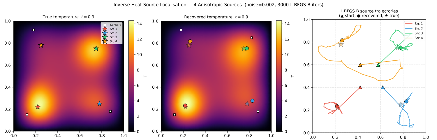
python examples/inverse_heat_source.py
Core architecture
The framework is built around SinusoidalBasis -- the analytical
derivative engine:
| Class | Purpose |
|---|---|
SinusoidalBasis |
Evaluates basis functions and arbitrary-order derivatives in O(1) via the cyclic identity |
BasisCache |
Pre-computes sin(Z)/cos(Z) once, reuses across multiple derivative evaluations |
DiffOperator / Op |
Symbolic linear differential operators that compose via +, -, scalar * |
FeatureBasis |
Adapter for non-sinusoidal solvers (e.g. PIELM with tanh) |
FastLSQSolver |
Manages feature blocks; exposes .basis for all derivative computations |
LearnableFastLSQ |
Differentiable solver with learnable bandwidth via reparameterisation trick |
How it works
-
Basis construction. Given collocation points x, construct a
SinusoidalBasiswith random weights W and biases b. -
Analytical derivatives. Exploit the cyclic derivative identity: the n-th derivative of sin(z) cycles through {sin, cos, -sin, -cos} with monomial weight prefactors. Any mixed partial
D^alpha phi_j(x)is computed in O(1) -- no computational graph, no automatic differentiation. -
PDE assembly. Define the differential operator symbolically with
Op(e.g.Op.laplacian(d=2)) and apply it to the basis to get the system matrixA. -
Linear solve. Solve
A beta = bvia least squares (optionally Tikhonov-regularised). -
Newton iteration (nonlinear). Linearise the PDE residual, solve
J delta_beta = -Rwith backtracking line search, and repeat.
Adding your own PDE
Define a problem class and use solver.basis to build the linear system:
import torch, numpy as np
from fastlsq import solve_linear, Op
from fastlsq.geometry import sample_box, sample_boundary_box

class MyPoisson2D:
    def __init__(self):
        self.name = "My Poisson"
        self.dim = 2
        self.pde_op = -Op.laplacian(d=2)

    def exact(self, x):
        return torch.sin(np.pi * x[:, 0:1]) * torch.sin(np.pi * x[:, 1:2])

    def exact_grad(self, x):
        sx, cx = torch.sin(np.pi * x[:, 0:1]), torch.cos(np.pi * x[:, 0:1])
        sy, cy = torch.sin(np.pi * x[:, 1:2]), torch.cos(np.pi * x[:, 1:2])
        return torch.cat([np.pi * cx * sy, np.pi * sx * cy], dim=1)

    def source(self, x):
        return 2 * np.pi**2 * self.exact(x)

    def get_train_data(self, n_pde=5000, n_bc=1000):
        x_pde = sample_box(n_pde, self.dim)
        f_pde = self.source(x_pde)
        x_bc = sample_boundary_box(n_bc, self.dim)
        u_bc = self.exact(x_bc)
        return x_pde, [(x_bc, u_bc)], f_pde

    def build(self, solver, x_pde, bcs, f_pde):
        basis = solver.basis
        cache = basis.cache(x_pde)
        A_pde = self.pde_op.apply(basis, x_pde, cache=cache)
        As, bs = [A_pde], [f_pde]
        for (x_bc, u_bc) in bcs:
            As.append(100.0 * basis.evaluate(x_bc))
            bs.append(100.0 * u_bc)
        return torch.cat(As), torch.cat(bs)

    def get_test_points(self, n=5000):
        return sample_box(n, self.dim)

result = solve_linear(MyPoisson2D(), scale=5.0)
See examples/add_your_own_pde.py for the complete tutorial.
Features
- Analytical derivative engine:
SinusoidalBasiscomputes arbitrary-order derivatives exactly in O(1) -- the foundation of the entire framework - Symbolic PDE operators: Compose differential operators with
Op(Laplacian, wave, Helmholtz, biharmonic, custom) via intuitive arithmetic - High-level API: Solve PDEs in one line with
solve_linear()andsolve_nonlinear() - Learnable bandwidth:
LearnableFastLSQoptimises the bandwidth (scalar or anisotropic) via reparameterisation - Auto-tuning: Automatic scale selection via grid search
- Built-in plotting: Solution visualization, convergence plots, spectral sensitivity
- Geometry samplers: Box, ball, sphere, interval, custom samplers
- Diagnostics: Problem validation, conditioning checks, error detection
- Export utilities: NumPy conversion, checkpoint saving/loading
- PyTorch Lightning: Integration for training loops
- 20+ benchmark problems: Linear, nonlinear, and regression-mode PDEs
Paper
The full preprint is available on arXiv
Citing this work
If you use FastLSQ in your research, please cite:
@misc{sulc2026solvingpdesshotfourier,
      title={Solving PDEs in One Shot via Fourier Features with Exact Analytical Derivatives},
      author={Antonin Sulc},
      year={2026},
      eprint={2602.10541},
      archivePrefix={arXiv},
      primaryClass={math.NA},
      url={https://arxiv.org/abs/2602.10541},
}
Building for PyPI
To build and upload a new release to PyPI:
# Install build tools
pip install build twine

# Bump version in pyproject.toml if needed, then build
python -m build

# Upload to PyPI (requires PyPI API token)
twine upload dist/*
For Test PyPI first: twine upload --repository testpypi dist/*
License
This project is licensed under the MIT License -- see LICENSE for details.


Download files
Download the file for your platform. If you're not sure which to choose, learn more about installing packages.
Source Distribution
Built Distribution
Filter files by name, interpreter, ABI, and platform.
If you're not sure about the file name format, learn more about wheel file names.
Copy a direct link to the current filters
File details
Details for the file fastlsq-0.1.1.tar.gz.
File metadata
- Download URL: fastlsq-0.1.1.tar.gz
- Upload date:
- Size: 340.1 kB
- Tags: Source
- Uploaded using Trusted Publishing? No
- Uploaded via: twine/6.2.0 CPython/3.9.18
File hashes
| Algorithm | Hash digest | |
|---|---|---|
| SHA256 |
c4d6f74e8a4cace86f92e083e248a719a77aca5e96c7cc42753ede6da246baa6
|
|
| MD5 |
1f36e1108afd9bc72766e403eeead898
|
|
| BLAKE2b-256 |
52cac03c2fa239cb093132d7c1592dad15d559e4c0f94c5376c4023f006f6493
|
File details
Details for the file fastlsq-0.1.1-py3-none-any.whl.
File metadata
- Download URL: fastlsq-0.1.1-py3-none-any.whl
- Upload date:
- Size: 41.5 kB
- Tags: Python 3
- Uploaded using Trusted Publishing? No
- Uploaded via: twine/6.2.0 CPython/3.9.18
File hashes
| Algorithm | Hash digest | |
|---|---|---|
| SHA256 |
2d2ca5c754b8d3933630f306f01c0d9420b19e9a14f19bfc7d176ecceb5203cd
|
|
| MD5 |
e5471ef0d77533d59710d0e4103610e1
|
|
| BLAKE2b-256 |
290c403c26eacd264d39d9a7a6301c4363bf5d58731b65a5de18ed0d11c72278
|


