HLR - Hierarchical Linear Regression for Python

Project description
HLR - Hierarchical Linear Regression in Python


HLR is a simple Python package for running hierarchical regression. It was created because there wasn't any good options to run hierarchical regression without using programs like SPSS.
Features
It is built to work with Pandas dataframes, uses SciPy and statsmodels for all statistics and regression functions, and runs diagnostic tests for testing assumptions while plotting figures with matplotlib and seaborn.
- Easy model creation and initiation with input data as Pandas dataframes
- Diagnostic tests and plots for checking assumptions:
- Independence of Residuals
- Durbin Watson Test
- Linearity
- Pearson's Correlations for DV and each IV
- Rainbow Test
- Plot: Studentised Residuals vs Fitted Values
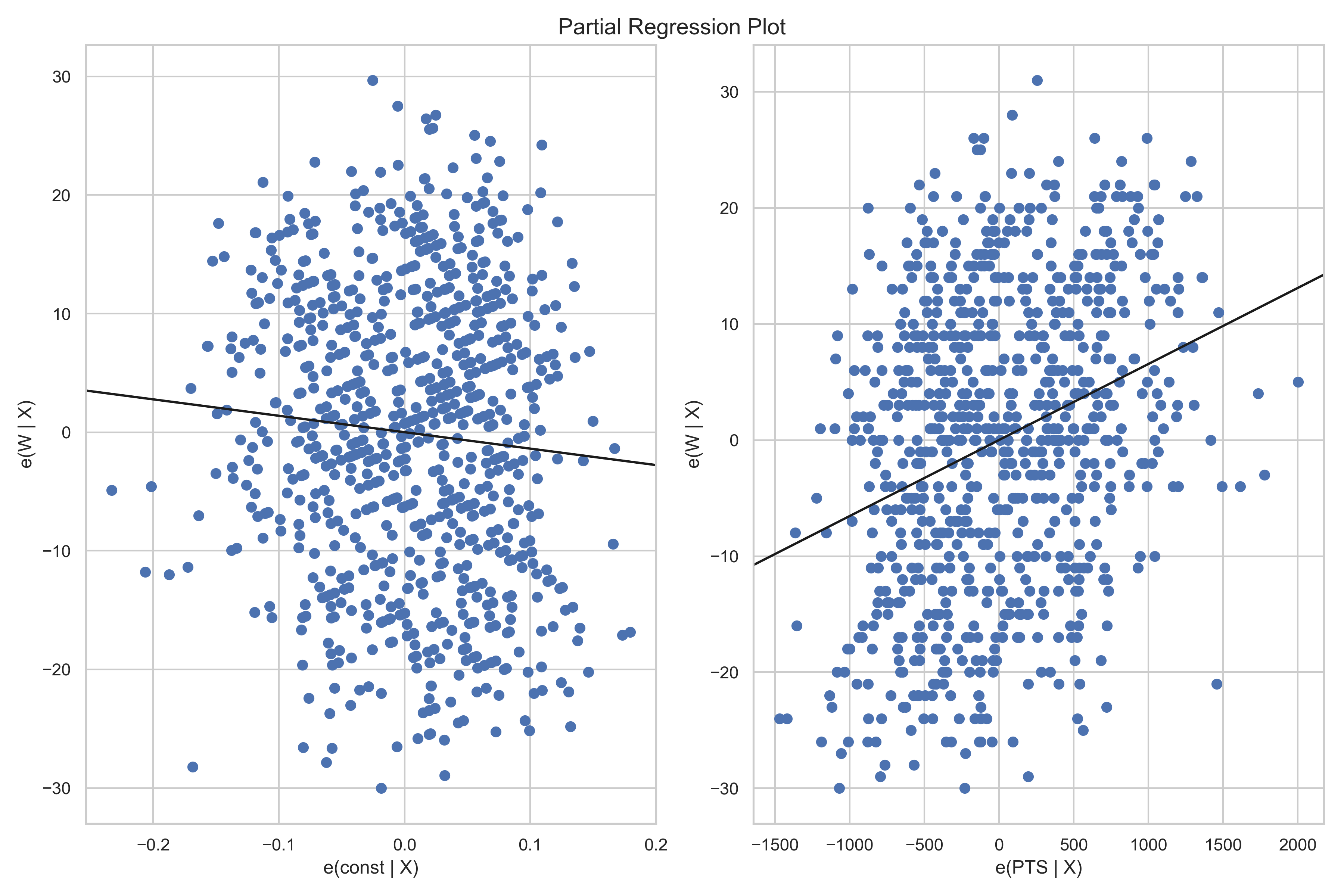
- Plot: Partial Regression Plots)
- Homoscedasticity
- Breusch Pagan Test
- F-test
- Goldfeld Quandt Test
- Plot: Studentised Residuals vs Fitted Values
- Multicollinearity
- Pairwise Correlations between DVs
- Variance Inflation Factor
- Outliers/Influence
- Standardised Residuals (> -3 & < +3)
- Cook's Distance
- Plot: Boxplot of Standardised Residuals
- Plot: Influence Plot with Cook's Distance
- Normality
- Mean of Residuals (approx = 0)
- Shapiro-Wilk Test
- Plot: Normal QQ Plot of Residuals)*
- Independence of Residuals
Installation
HLR is meant to be used with Python 3.x and has been tested on Python 3.7-3.9.
Dependencies
User installation
To install HLR, run this command in your terminal:
pip install hlr
This is the preferred method to install HLR, as it will always install the most recent stable release.
If you don’t have pip installed, this Python installation guide can guide you through the process.
Usage
Quick start
An example Jupyter Notebook can be found in 'example' subfolder with a sample dataset. You can also just run the code below.
import pandas as pd
import HLR

nba = pd.read_csv('example/NBA_train.csv')

# List of dataframes of predictor variables for each step
X = [nba[['PTS']],
     nba[['PTS', 'ORB']],
     nba[['PTS', 'ORB', 'BLK']]]

# List of predictor variable names for each step
X_names = [['points'],
           ['points', 'offensive_rebounds'],
           ['points', 'offensive_rebounds', 'blocks']]

# Outcome variable as dataframe
y = nba[['W']]

# Create a HLR model with diagnostic tests, run and save the results
model = HLR.HLR_model(diagnostics=True, showfig=True, save_folder='results', verbose=True)
model_results, reg_models = model.run(X=X, X_names=X_names, y=y)
model.save_results(filename='nba_results', show_results=True)
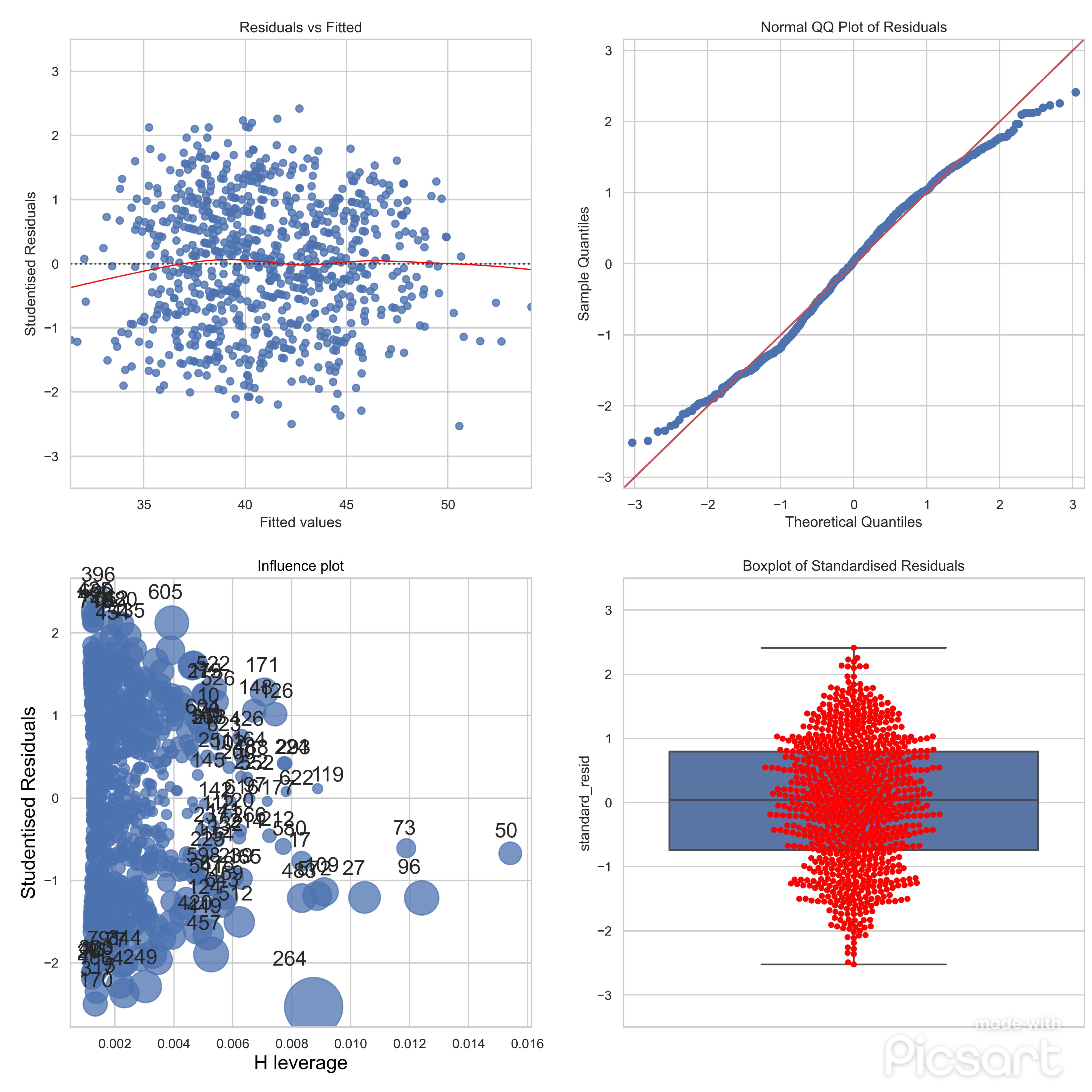
Diagnostics output
Diagnostic tests and plots for the step 1 of the model mentioned above.
Diagnostic tests - step1

Independence of Residuals = PASSED (Durbin-Watson Test)
Linearity = PASSED (Non-sig. linear relationship between DV and each IV)
Linearity = PASSED (Rainbow Test)
Homoscedasticity = FAILED (Bruesch Pagan Test)
Homoscedasticity = FAILED (F-test for residual variance)
Homoscedasticity = PASSED (Goldfeld Quandt Test)
Multicollinearity = PASSED (High Pairwise correlations)
Multicollinearity = PASSED (High Variance Inflation Factor)
Outliers/Leverage/Influence = PASSED (Extreme Standardised Residuals)
Outliers/Leverage/Influence = PASSED (Large Cook's Distance)
Normality = PASSED (Mean of residuals not approx = 0)
Normality = FAILED (Shapiro-Wilk Test)

FURTHER INSPECTION REQUIRED -> 1/3 tests passed for assumption - Homoscedasticity
FURTHER INSPECTION REQUIRED -> 1/2 tests passed for assumption - Normality

...
 |
 |
|---|
Results output
HLR model output of all three steps of the model mentioned above.
| Step | Predictors | N (observations) | DF (residuals) | DF (model) | R-squared | F-value | P-value (F) | SSE | SSTO | MSE (model) | MSE (residuals) | MSE (total) | Beta coefs | P-values (beta coefs) | Failed assumptions (check!) | R-squared change | F-value change | P-value (F change) | |
|---|---|---|---|---|---|---|---|---|---|---|---|---|---|---|---|---|---|---|---|
| 0 | 1 | [points] | 835.0 | 833.0 | 1.0 | 0.089297 | 81.677748 | 1.099996e-18 | 123292.827686 | 135382.0 | 12089.172314 | 148.010597 | 162.328537 | {'Constant': -13.846261266053896, 'points': 0.... | {'Constant': 0.023091997486255577, 'points': 1... | [Homoscedasticity, Normality] | NaN | NaN | NaN |
| 1 | 2 | [points, offensive_rebounds] | 835.0 | 832.0 | 2.0 | 0.168503 | 84.302598 | 4.591961e-34 | 112569.697267 | 135382.0 | 11406.151367 | 135.300117 | 162.328537 | {'Constant': -14.225561767669713, 'points': 0.... | {'Constant': 0.014660145903221372, 'points': 1... | [Normality, Multicollinearity] | 0.079206 | 79.254406 | 3.372595e-18 |
| 2 | 3 | [points, offensive_rebounds, blocks] | 835.0 | 831.0 | 3.0 | 0.210012 | 73.638176 | 3.065838e-42 | 106950.174175 | 135382.0 | 9477.275275 | 128.700571 | 162.328537 | {'Constant': -21.997353037483723, 'points': 0.... | {'Constant': 0.00015712851466562279, 'points':... | [Normality, Multicollinearity, Outliers/Levera... | 0.041509 | 43.663545 | 6.962046e-11 |
Documentation
Visit the documentation for more information. https://hlr-hierarchical-linear-regression.readthedocs.io
Citation
Please use Zenodo DOI for citing the package in your work.
Example
Toomas Erik Anijärv, & Rory Boyle. (2023). teanijarv/HLR: v0.1.4 (v0.1.4). Zenodo. https://doi.org/10.5281/zenodo.7683808
@software{toomas_erik_anijarv_2023_7683809,
  author       = {Toomas Erik Anijärv and
                  Rory Boyle},
  title        = {teanijarv/HLR: v0.1.4},
  month        = feb,
  year         = 2023,
  publisher    = {Zenodo},
  version      = {v0.1.4},
  doi          = {10.5281/zenodo.7683809},
  url          = {https://doi.org/10.5281/zenodo.7683808}
}
Development
HLR was created by Toomas Erik Anijärv using original code by Rory Boyle. The package is maintained by Toomas during his spare time, thereby contributions are more than welcome!
This program is provided with no warranty of any kind and it is still under heavy development. However, this code has been checked and validated against multiple same analyses conducted in SPSS.
To-do
Would be great if someone with more experience with packages would contribute with testing and the whole deployment process. Also, if someone would want to write documentation, that would be amazing.
- Documentation
- More thorough testing
Contributors
Toomas Erik Anijärv Rory Boyle
Credits
This package was created with Cookiecutter and the audreyr/cookiecutter-pypackage project template.
======= History
0.1.0 (2023-02-24)
- First release on PyPI.
0.1.4 (2023-03-9)
- Fixed pairwise correlations threshold for multicollinearity assumption testing (0.3 -> 0.7)
- Fixed partial regression plots fixed figure size
- Added titles to diagnostic plots
- Fixed the VIF to match with SPSS output by adding the constant to X
Release history Release notifications | RSS feed


Download files
Download the file for your platform. If you're not sure which to choose, learn more about installing packages.
Source Distribution
Built Distribution
Filter files by name, interpreter, ABI, and platform.
If you're not sure about the file name format, learn more about wheel file names.
Copy a direct link to the current filters
File details
Details for the file HLR-0.1.4.tar.gz.
File metadata
- Download URL: HLR-0.1.4.tar.gz
- Upload date:
- Size: 1.1 MB
- Tags: Source
- Uploaded using Trusted Publishing? No
- Uploaded via: twine/4.0.2 CPython/3.9.13
File hashes
| Algorithm | Hash digest | |
|---|---|---|
| SHA256 |
3a844389d808bd93d72c4eac025397be2878fcfdbc0d309dfd86dc204f09b472
|
|
| MD5 |
45b48161d2d95e3d1eb58b867225e3a3
|
|
| BLAKE2b-256 |
c2819c78e7bedd76ef5884009ebb0dc06c785b8e0cb6e7de9f5652a3b20189c9
|
File details
Details for the file HLR-0.1.4-py2.py3-none-any.whl.
File metadata
- Download URL: HLR-0.1.4-py2.py3-none-any.whl
- Upload date:
- Size: 17.6 kB
- Tags: Python 2, Python 3
- Uploaded using Trusted Publishing? No
- Uploaded via: twine/4.0.2 CPython/3.9.13
File hashes
| Algorithm | Hash digest | |
|---|---|---|
| SHA256 |
c79643aeb3ef9de784ea869325f6097f84f687d0cd041c37d3d44eb9ea1f53b7
|
|
| MD5 |
e0ab0da53fc641ceb7d2eabfca01e853
|
|
| BLAKE2b-256 |
da9ef591b05d6e1319ae9576b8246477af3a85daa8efa55968b1273aa1f3260c
|


