MANTA-Ray (Modified Absorption of Non-spherical Tiny Aggregates in the Rayleigh regime) is a model that calculates the absorption efficiency and absorption cross-section of fractal aggregates.

Project description

MANTA-Ray (Modified Absorption of Non-spherical Tiny Aggregates in the Rayleigh regime) is a model that calculates the absorption efficiency and absorption cross-section of fractal aggregates. It is a very powerful and fast tool that can be used to estimate the amount of absorption that occurs in dust and haze particles of any shape, provided that the electromagnetic radiation is in the Rayleigh regime (see below for strict definition), often in the context of planetary atmospheres or protoplanetary disks. It obtains values within 10-20% of those calculated by a rigorous benchmark model (the discrete dipole approximation), but is $10^{13}$ times faster. It is provided here as two python functions. For full details of the methodology, or if the code is useful in your project, please cite the paper below:
"MANTA-Ray: Supercharging Speeds for Calculating the Optical Properties of Fractal Aggregates in the Long-Wavelength Limit" (2024), Lodge, M.G., Wakeford H.R., and Leinhardt, Z.M.
Getting started
The easiest way to run MANTA-Ray is to install it into your python environment using pip:
pip install MANTA_Ray_optics
Then import the functions into your python code and try an example calulation (IMPORTANT: Note the use of underscores _ instead of hyphens - for importing the module, as suggested by the python PEP 8 style guide):
# import the module
from MANTA_Ray_optics import MANTA_Ray

# set the input variables
wavelength = 100   # in um
radius = 0.5   # in um
d_f = 1.8
n = 3
k = 0.5

# calculate Q_abs
Q_abs = MANTA_Ray.find_Q_abs(wavelength, radius, d_f, n, k)

print(Q_abs)
If MANTA-Ray installed correctly, you should see the value:
0.021153387751343056
The inputs to the functions are:
- wavelength: the wavelength ($\lambda$) of the electromagnetic radiation (in μm).
- radius: the particle radius ($R$) (in μm) -- see note below*.
- d_f: the fractal dimension ($d_f$) of the aggregate. The code has been tested for values between $d_f=$ 1.2 (linear) and 2.7 (compact). See section "The Model" below for more details.
- n: the real component of refractive index
- k: the imaginary component of refractive index
*Because the aggregates are non-spherical, they do not have a radius. To represent the physical size of the particle, we use the radius of a sphere that has exactly the same volume as the fractal aggregate (i.e. the radius if the aggregate material was squashed/compacted into a sphere).
The example above determines the absorption efficiency of an aggregate of fractal dimension 1.8, with a radius of 0.5 μm, at a wavelength of 100 μm, and assuming a material refractive index $m=n+k$ i = 3 + 0.5 i. Note that to be in the Rayleigh regime, and for this theory to work, it is assumed that $\lambda \geq 100R$, and the code will return an error message (and not proceed) if this condition is not met.
To use the functions, just provide the above inputs, strictly in that order. There are two functions in this package:
- find_Q_abs: calculates absorption efficiency $Q_{abs,MR}$ (Eq. 5 in Lodge et al. 2024)
- find_C_abs: calculates absorption cross-section (where $C_{abs}=Q_{abs} \pi R^2$)
Both functions use the same input variables:
Q_abs = MANTA_Ray.find_Q_abs(wavelength, radius, d_f, n, k)
C_abs = MANTA_Ray.find_C_abs(wavelength, radius, d_f, n, k)
If a pip install fails (or simply if you prefer), you could copy and paste the functions from MANTA_Ray.py directly into your code and use them as regular functions instead.
The Model
This section provides a brief overview of the model, but for a full explanation and more details, please read Lodge et al. 2024.
Transmission Electron Microscope (TEM) images of solid matter in Earth's atmosphere shows that they often form very complex shapes, which we call fractal aggregates. Their exact shape depends on the material and conditions under which they form. Typically, we characterise them by a single number -- their fractal dimension $d_f$:
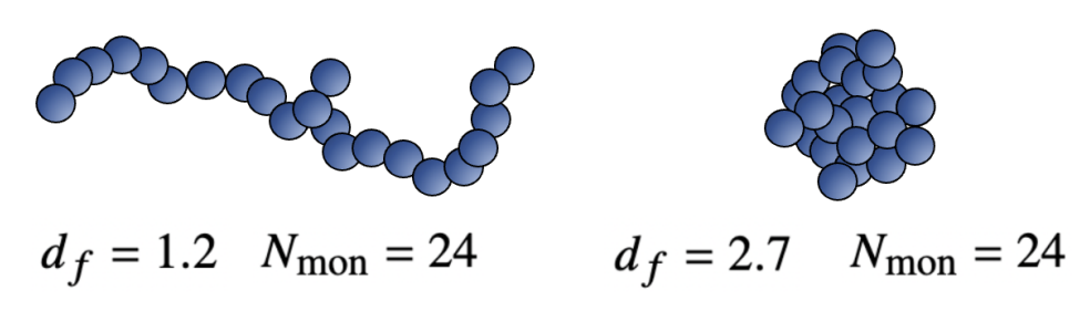
In the image above the two aggregates are both composed of 24 "monomers" (individual spheres), but in different arrangements. These shapes are characterised in many optical models by $d_f$ which is a number between 1 (representing a straight line) and 3 (compact and perfectly spherical).
Modelling the optical properties of complex shapes is difficult, and Mie theory is often used (which assumes that the particles are spherical). However, this can often be a significant underestimate of the amount of absorption (by factors of up to 1,000 -- see Lodge et al. 2024). Calculating the optical properties for the true aggregate shape can be done using a rigorous code such as the discrete dipole approximation (DDA -- Draine and Flatau, 1994), but this is usually incredibly time consuming (and unfeasible for use in forward models that wish to study many wavelengths/particle sizes). In contrast, MANTA-Ray estimates absorption cross-sections with average accuracies of 10-20% compared to DDA, but $10^{13}$ times faster. It works for any wavelength, particle size, and refractive index $m$ within 1+0.01i< $m$ <11+11i. It is strictly only for use in the Rayleigh Regime (where the wavelength $\lambda$ is significantly larger than the radius $R$ of a sphere of equivalent volume to the aggregate -- here we define this regime as $\lambda \geq 100R$).
The MANTA-Ray model uses the following equation to determine the absorption efficiency $Q_\mathrm{abs}$:
$Q_\mathrm{ext} = \chi \frac{8 \pi R}{\lambda} \mathrm{Im} \left(\frac{m^2 - 1}{m^2 + 1} \right)$
Where the modification factor $\chi$ is given by:
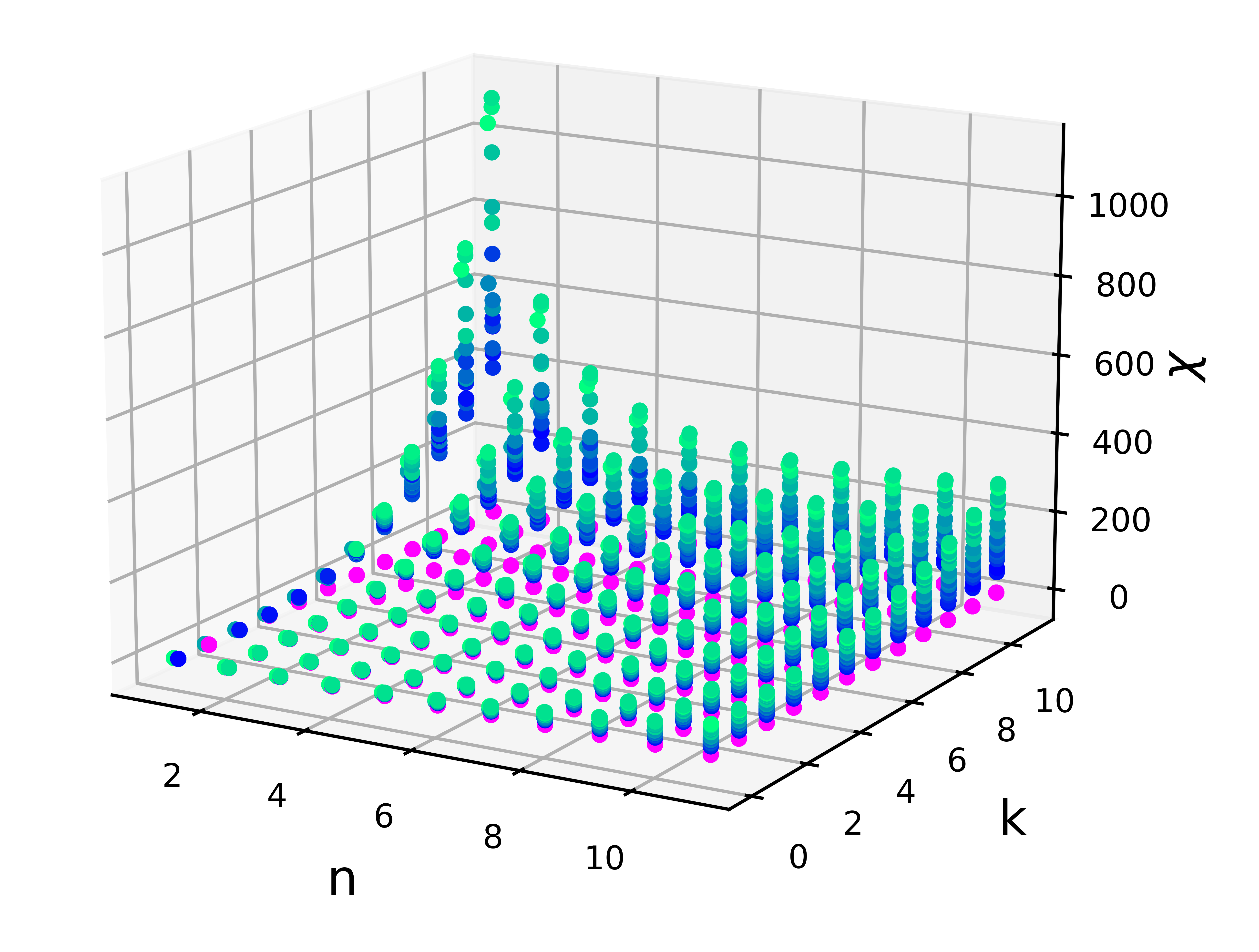
$\chi = a_0 + a_1 n +a_2 k + a_3 n^2 + a_4 nk + a_5 k^2$
And the coefficients $a_0$ - $a_5$, are calculated using the methodology in Lodge et al. (2024).
Lookup table functionality
In MANTA-Ray v2.0, we provide functionality to interpolate between and extrapolate from the original DDA dataset using a thin plate spine within the RBF interpolator of SciPy. This allows users to estimate DDA results from the dataset that was used to build MANTA-Ray, in a more precise way than using the quadratic function from the regular model, for cases where extreme accuracy is important. Users can choose a different value for d_f, n, and k, and the code will interpolate using the dataset below to find X rather than using the quadratic model from the paper (see above). To use this functionality, simply add the variable lookup=True to the function call, e.g.:
Q_abs = MANTA_Ray.find_Q_abs(wavelength, radius, d_f, n, k, lookup=True)
C_abs = MANTA_Ray.find_C_abs(wavelength, radius, d_f, n, k, lookup=True)
The default value for this parameter is lookup=False, which reverts to using the quadratic model from Lodge et al. (2024).
Release history Release notifications | RSS feed


Download files
Download the file for your platform. If you're not sure which to choose, learn more about installing packages.
Source Distribution
Built Distribution
Filter files by name, interpreter, ABI, and platform.
If you're not sure about the file name format, learn more about wheel file names.
Copy a direct link to the current filters
File details
Details for the file manta_ray_optics-2.0.0.tar.gz.
File metadata
- Download URL: manta_ray_optics-2.0.0.tar.gz
- Upload date:
- Size: 17.6 kB
- Tags: Source
- Uploaded using Trusted Publishing? No
- Uploaded via: twine/5.1.1 CPython/3.9.7
File hashes
| Algorithm | Hash digest | |
|---|---|---|
| SHA256 |
56e1ca4111e3a9771abacc9d3dc9bcb5d53238a24c9c61c44385be17d964c680
|
|
| MD5 |
30e3fec71510b8aef0e2129edba92722
|
|
| BLAKE2b-256 |
cd5a663e154bc1654ab18187b46c7317ba5f732ba8acb3560055dc010263e300
|
File details
Details for the file manta_ray_optics-2.0.0-py3-none-any.whl.
File metadata
- Download URL: manta_ray_optics-2.0.0-py3-none-any.whl
- Upload date:
- Size: 18.3 kB
- Tags: Python 3
- Uploaded using Trusted Publishing? No
- Uploaded via: twine/5.1.1 CPython/3.9.7
File hashes
| Algorithm | Hash digest | |
|---|---|---|
| SHA256 |
288a22ac750df5a42feb0a274dff85ec4b774b85fff538622243559d5fd10334
|
|
| MD5 |
64ba4368b40a969ca717ab93e9646ebb
|
|
| BLAKE2b-256 |
7e7a0cba4bc01ae0817ac96bae01a44e347cde581526ab1dc1d747c53d14caca
|


