
MultiMM: An OpenMM-based software for whole genome 3D structure reconstruction
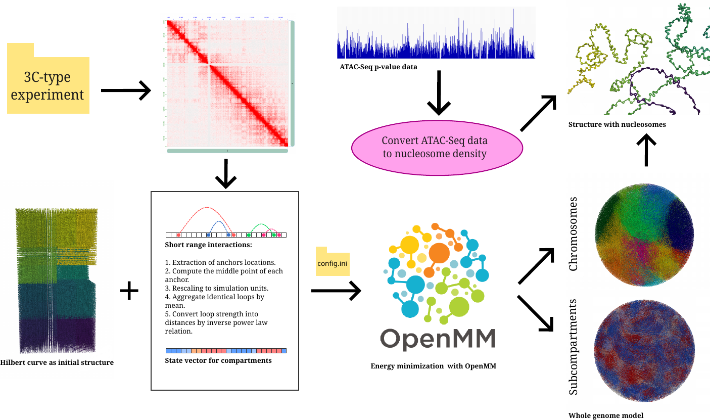
MultiMM is an OpenMM model designed for modeling the 3D structure of the whole human genome. Its distinguishing feature is that it is multiscale, meaning it aims to model different levels of chromatin organization, from smaller scales (nucleosomes) to the level of chromosomal territories. The algorithm is both fast and accurate. A key feature enabling its speed is GPU parallelization via OpenMM, along with smart assumptions that assist the optimizer in finding the global minimum. One such fundamental assumption is the use of a Hilbert curve as the initial structure. This helps MultiMM to converge faster because the initial structure is already highly compacted.
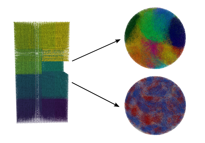
After running the MultiMM model, users obtain a genome-wide structure. Users can color different chromosomes or compartments, or they can visualize individual chromosomes separately. MultiMM is simple to use, as it is based on modifying a single configuration file. Here we explain its usage.
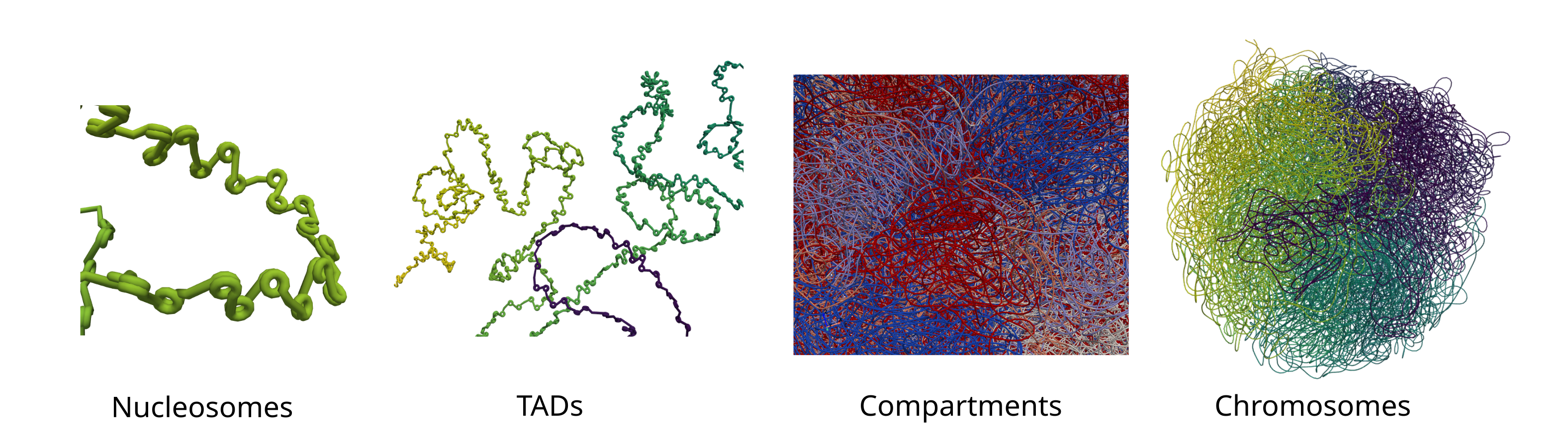
The workflow of MultiMM is illustrated in the following schematic. The user first provides a set of interactions from a 3C-type experiment, representing chromatin loops, and optionally supplies compartment annotations. The user can also specify a region or chromosome of interest. MultiMM then imports an initial structure, performs basic preprocessing on the input data, and applies a force field corresponding to the provided interactions. All simulation parameters and user preferences must be specified in the config.ini file. Afterward, the software generates the 3D chromatin structures, and, if ATAC-Seq data are provided, applies nucleosome interpolation to refine the model.
Key Features
- OpenMM based.
- User-friendly software available via PyPI.
- Efficient simulation of chromatin interactions using 3D conformations.
- Can simulate the scales of nucleosomes, TADs, compartments, chromosomal territories and interactions with lamina. Scalable simulations across different force fields and resolution levels.
- Compatible with modern GPU-accelerated simulation libraries. CPU acceleration can also be done.
- Possibility of creation of ensembles of 3D structures of chromatin.
About Operating Systems
MultiMM has been tested primarily on Linux-based operating systems, with successful tests in Ubuntu, Debian, and Red Hat-based distributions. It is also possible to run it on macOS, though without CUDA support, which is helpful for accelerating computations. We do not recommend running MultiMM on Windows systems.
Installation
MultiMM can be easily installed with pip:
pip install MultiMM
PyPI software: https://pypi.org/project/MultiMM/.
Model Overview
We model chromatin as a coarse-grained polymer where the total energy $E$ is decomposed into a set of physically motivated interaction terms capturing polymer mechanics, epigenetic organization, and structural constraints. Each term encodes a distinct biological mechanism, allowing the model to reproduce both local polymer behavior and large-scale genome organization such as compartments and loops.
At a generic level, the system is governed by a total energy of the form
$$E = E_{\text{backbone}} + E_{\text{block-copolymer}} + E_{\text{loops}} + E_{\text{excluded}} + E_{\text{confinement}} + E_{\text{chromosomal}}$$
where each contribution controls a different aspect of chromatin folding:
- $E_{\text{backbone}}$: enforces polymer connectivity and stiffness through bonded and angular interactions, ensuring a realistic chain-like structure
- $E_{\text{block-copolymer}}$: captures compartment and subcompartment segregation via state-dependent attractive interactions between beads
- $E_{\text{loops}}$: introduces long-range constraints between genomic loci, mimicking loop extrusion or experimentally observed contacts
- $E_{\text{excluded}}$: accounts for steric repulsion, preventing unphysical overlaps between beads
- $E_{\text{confinement}}$: imposes nuclear geometry through spherical confinement and lamina interactions
- $E_{\text{chromosomal}}$: promotes large-scale organization such as chromosome territories and global compaction
Together, these terms define a minimal yet flexible energy landscape where local polymer physics and global genomic features emerge in a unified framework.
Polymer Backbone
The backbone contribution $E_{\text{backbone}}$ encodes the connectivity and local rigidity of the polymer chain. It is composed of two standard terms: harmonic bonds enforcing nearest-neighbor distances, and harmonic angle potentials controlling chain stiffness.
The bond (connectivity) term is given by
$$E_{\text{bond}} = \sum_{i} \frac{k_b}{2} \left( r_{i,i+1} - r_0 \right)^2$$
where $r_{i,i+1} = |\mathbf{r}_{i+1} - \mathbf{r}_i|$ is the distance between consecutive beads, $r_0$ is the equilibrium bond length, and $k_b$ is the bond stiffness. This term ensures that the polymer remains connected and fluctuates around a preferred contour length.
The stiffness (bending) term is defined as
$$E_{\text{angle}} = \sum_{i} \frac{k_\theta}{2} \left( \theta_i - \theta_0 \right)^2$$
where $\theta_i$ is the angle formed by three consecutive beads $(i, i+1, i+2)$, $\theta_0$ is the preferred angle, and $k_\theta$ controls the bending rigidity. This term penalizes sharp bends and sets the persistence length of the polymer.
Altogether, the backbone energy reads
$$E_{\text{backbone}} = E_{\text{bond}} + E_{\text{angle}}$$
which corresponds to a discretized worm-like chain model with harmonic stretching and bending fluctuations.
Loop Interactions
The loop contribution $E_{\text{loops}}$ introduces long-range interactions between pairs of beads $(m,n)$, representing loop extrusion or experimentally detected contacts. Each loop acts as an effective tether that constrains the spatial distance between distant genomic loci.
The default model uses a harmonic potential
$$E_{\text{loops}}^{\text{harmonic}} = \sum_{(m,n)} \frac{k}{2} \left( r_{mn} - r_0 \right)^2$$
where $r_{mn} = |\mathbf{r}_n - \mathbf{r}_m|$, $r_0$ is the preferred loop length, and $k$ is the stiffness. This formulation strongly penalizes deviations from $r_0$, effectively enforcing fixed-distance loops and providing a simple baseline model.
To allow more physical flexibility, two alternative bounded interactions are introduced. The first is a soft FENE-like potential
$$E_{\text{loops}}^{\text{fene}} = \sum_{(m,n)} \frac{k (r_{mn} - r_0)^2}{1 + \alpha (r_{mn} - r_0)^2}$$
which behaves harmonically near equilibrium but saturates at large extensions. This avoids unphysical divergence and models loops as extensible but finite-strength tethers.
The second alternative is a Gaussian tether
$$E_{\text{loops}}^{\text{gaussian}} = \sum_{(m,n)} k \left( 1 - e^{-(r_{mn} - r_0)^2 / \sigma^2} \right)$$
which defines a fully smooth, bounded potential well. Close to $r_0$ it is approximately harmonic, while at large distances it saturates to a constant energy, effectively allowing loop breaking without instability.
Block Copolymer Compartmentalization
The block-copolymer contribution $E_{\text{block}}$ encodes epigenetic segregation via state-dependent pairwise interactions. Each bead carries a label $s_i$ representing its compartment or subcompartment identity. These labels selectively activate interactions, driving chromatin phase separation into distinct domains.
Compartment level (A/B): Interactions follow a Gaussian attractive potential:
E_{\text{comp}} = -\sum \epsilon(s_i,s_j) \exp\left( -\frac{r_{ij}^2}{2r_c^2} \right)
where $r_{ij}$ is the distance between beads and $r_c$ is the interaction range. The coupling $\epsilon(s_i,s_j)$ is attractive for like compartments (A–A, B–B) and weak or repulsive otherwise, reproducing large-scale A/B segregation seen in Hi-C data.
Subcompartment level: The model is extended to multiple epigenetic states $\alpha,\beta$:
E_{\text{sub}} = -\sum \epsilon_{\alpha\beta} \exp\left( -\frac{r_{ij}^2}{2r_{sc}^2} \right) \quad \text{for } s_i=\alpha,\ s_j=\beta
where $r_{sc}$ controls the shorter interaction range. This promotes finer microphase separation inside A/B compartments, creating richer internal chromatin organization.
At the chromosome level, a weak self-attraction is introduced to promote territorial segregation:
E_{\text{chrom}} = \sum \delta_{\chi_i,\chi_j} V(r_{ij})
where $\chi_i$ denotes chromosome identity and $V(r)$ is a soft attractive potential acting only between beads of the same chromosome. In the default polynomial form,
V(r) = dE \left(k_C r^4 - r^3 + r^2\right)
This stabilizes globular chromosome conformations and enhances intra-chromosomal clustering while suppressing inter-chromosomal mixing, supporting the emergence of chromosome territories.
Beyond the Gaussian baseline, alternative kernels (e.g. Yukawa, power-law, and threshold interactions) modify the effective interaction range and decay profile, allowing systematic exploration of how the functional form of epigenetic attraction shapes chromatin organization.
- The Yukawa form replaces the Gaussian decay with a screened Coulomb-like interaction
$$V(r) \sim -\frac{e^{-r/\lambda}}{r}$$
introducing a longer-ranged but exponentially screened attraction. This allows compartmental domains to communicate over larger genomic distances and can enhance domain coarsening.
- The power-law interaction
$$V(r) \sim -\frac{1}{r^\alpha + \epsilon}$$
removes a characteristic length scale entirely, producing scale-free interactions. This is useful for probing whether compartmental organization can emerge from purely algebraic long-range correlations.
- For subcompartments, the theta (contact) model
$$V(r) \sim -\Theta(r_c - r)$$
reduces interactions to a hard cutoff contact rule, where only sufficiently close loci interact. This provides a minimal, binary version of epigenetic attraction, useful as a null model for testing the necessity of smooth potentials.
- For chromosome-level organization, the alternatives modify the confinement landscape: Gaussian attraction produces smooth globular collapse, while the saturating form
$$V(r) \sim -\frac{1}{1 + k_C r^2}$$
limits the strength of long-range attraction, preventing over-collapse and allowing more flexible chromosome territories.
Nuclear Geometry and Lamina Interactions
The lamina-related contribution introduces spatial confinement and peripheral anchoring of specific chromatin states, effectively coupling genome organization to nuclear geometry.
The spherical container defines a soft nuclear boundary by penalizing excursions outside a radial shell. The energy is
$$E_{\text{container}} = C \sum_i \left[ \max(0, r_i - R_2)^2 + \max(0, R_1 - r_i)^2 \right]$$
where $r_i$ is the radial distance of bead $i$ from the nuclear center. This creates a confined annular domain between radii $R_1$ and $R_2$, representing the accessible nuclear volume and preventing unphysical collapse or escape.
On top of this geometric confinement, the lamina interaction introduces state-dependent attraction of B-type chromatin to the nuclear periphery:
$$E_{\text{lamina}} = - \sum_i B(s_i), V(r_i)$$
where $s_i$ is the compartment state and $B(s_i)$ selects B-compartment beads. The function $V(r)$ encodes different radial potentials depending on the model choice:
The sinusoidal shell (default) creates a sharp peripheral preference within the shell
$$V(r) = \sin^8\left(\frac{\pi (r - R_1)}{R_2 - R_1}\right) - 1$$
while Gaussian shells localize attraction around the two boundaries $R_1$ and $R_2$
$$V(r) \sim -\left[e^{-(r-R_1)^2/(2\sigma^2)} + e^{-(r-R_2)^2/(2\sigma^2)}\right]$$
The harmonic shell instead pulls B-chromatin toward the mid-shell radius $r_0=\frac{R_1+R_2}{2}$,
$$V(r) \sim (r - r_0)^2$$
and the logistic form creates smooth attractive walls near both boundaries using sigmoidal transitions.
Together, these terms implement a minimal physical model of nuclear architecture where confinement defines the available volume, and lamina attraction biases epigenetically marked chromatin toward the nuclear periphery.
Nucleosome Scale Interpolation
After coarse grained optimization, nucleosome positions are interpolated using a beads on the string zigzag model. Each nucleosome is represented as a helix with 1.65 DNA turns. The number of nucleosomes per bead is derived from normalized ATAC Seq signal, enforcing nucleosome rich regions in low accessibility chromatin.
Internal parameter definitions
All geometric and interaction scales are now derived from a single microscopic length scale, the polymer bond length $b_0 =$ POL_HARMONIC_BOND_R0, ensuring consistent density and eliminating arbitrary global normalization factors.
The nuclear confinement is modeled as a dense polymer globule with constant monomer density. In this regime, the outer nuclear radius follows the standard scaling law
$$ R_2 = b_0 N^{1/3}, $$
which enforces $N / R_2^3 \approx \text{const}$ and guarantees physically consistent compaction as system size changes. The inner compartment (nucleolus-like region) is defined via a fixed volume fraction $f$ of the nuclear volume, leading to
$$ R_1 = R_2 f^{1/3}. $$
This construction ensures that compartment organization scales in a volume-preserving manner rather than through independent geometric tuning.
The compartment interaction length scale $r_c$ (previously $r_{\text{comp}}$) is no longer tied to geometric confinement. Instead, it represents the physical decay length of short-range attractive interactions between chromatin compartments and nuclear structures. It is defined directly from the polymer bond length as
$$ r_c \sim \mathcal{O}(b_0), $$
typically chosen as a small multiple of $b_0$ (e.g. $r_c \approx 1.5 b_0$), ensuring that interactions remain local and comparable to nearest-neighbor connectivity along the polymer backbone.
Loop constraints are encoded through bond-specific equilibrium distances $r_0^{(i)}$, which may either be globally fixed or informed by experimental loop length data $d_i$. This introduces controlled heterogeneity in loop architecture:
$$ r_0^{(i)} \in (r_0^{\text{global}}, d_i), $$
allowing loops to interpolate between polymer-native scales and experimentally inferred constraints.
Each bead carries discrete state variables such as compartment identity $s_i$ and chromosome label $\chi_i$. These variables do not directly define geometry but modulate interactions through selection rules of the form
$$ E_{ij} \propto \delta(s_i, s_j) \quad E_{ij} \propto \delta(\chi_i, \chi_j), $$
ensuring that only compatible epigenetic or chromosomal states contribute to attractive or repulsive terms. Together, these elements couple polymer physics, nuclear confinement, and epigenetic structure into a unified multiscale chromatin framework.
Input Data
MultiMM relies on three types of datasets:
- Loop interactions in
bedpeformat (mandatory). - Compartmentalization data in
bedformat (optional). - ATAC-Seq p-value data in
.BigWigformat (optional).
Loops (bedpe file)
For loop interactions, users must provide a file describing interactions between anchor 1 and anchor 2, along with their strength.
The file must be in .bedpe format, contain 7 columns, and must not include a header.
chr10	100225000	100230000	chr10	100420000	100425000	95
chr10	100225000	100230000	chr10	101005000	101010000	56
chr10	101190000	101195000	chr10	101370000	101375000	152
chr10	101190000	101200000	chr10	101470000	101480000	181
chr10	101600000	101605000	chr10	101805000	101810000	152
The file can include interactions from all chromosomes; MultiMM will automatically handle them.
For single-cell data, users should prepare the file by setting the second and third columns identical (as well as the fifth and sixth columns) and set the strength value to 1.
Compartments
For (sub)compartment interactions, the file should be in the format produced by the CALDER software: https://github.com/CSOgroup/CALDER2. Users do not need to run CALDER specifically, but the file format must match. The file should contain at least the first four columns with chromosome, regions, and the subcompartment label. Example:
chr1	700001	900000	A.1.2.2.2.2.2.2	0.875	.	700001	900000	#FF4848
chr1	900001	1400000	A.1.1.1.1.2.1.1.1.1.1	1	.	900001	1400000	#FF0000
chr1	1400001	1850000	A.1.1.1.1.2.1.2.2.2.1	1	.	1400001	1850000	#FF0000
chr1	1850001	2100000	B.1.1.2.2.1.2.1	0.5	.	1850001	2100000	#DADAFF
Nucleosomes
For ATAC-Seq data, users must provide a BigWig file containing p-values. The pyBigWig library is required to read BigWig files. Note: pyBigWig is not compatible with Windows systems.
Definition of a region based on a gene (optional)
To model a genomic region around a specific gene, you can load a .tsv file containing gene information. Specify either the gene name or the gene ID.
The .tsv file should be formatted as follows:
gene_id	gene_name	chromosome	start	end
ENSG00000160072	ATAD3B	chr1	1471765	1497848
ENSG00000279928	DDX11L17	chr1	182696	184174
ENSG00000228037		chr1	2581560	2584533
ENSG00000142611	PRDM16	chr1	3069168	3438621
ENSG00000284616		chr1	5301928	5307394
ENSG00000157911	PEX10	chr1	2403964	2413797
ENSG00000269896		chr1	2350414	2352820
ENSG00000228463		chr1	257864	359681
ENSG00000260972		chr1	5492978	5494674
ENSG00000224340		chr1	10054445	10054781
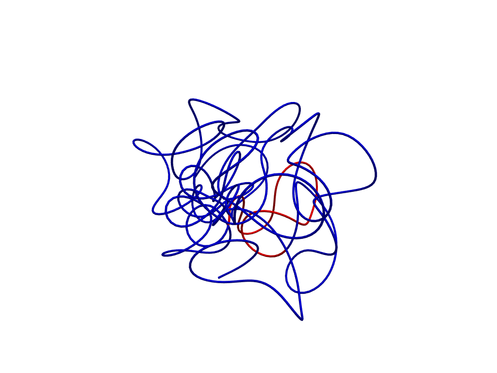
In case that you specify the gene, MultiMM will output a visualization with the gene as well. For example, in the folowing region we can see the polymer structure that is modelled (around the gene) and the gene with red color.
The MultiMM model targets the gene file automatically, so you do not have to provide it. However, you can optionally change it.
Note: Currently, MultiMM is designed to work with human genome data. While it may be possible to run the code on other organisms with additional debugging and modifications, full support for other species is planned for future versions. MultiMM can process various types of datasets. It is capable of calling loops from a range of experiments, including Hi-C, scHi-C, ChIA-PET, and Hi-ChIP. However, we cannot guarantee that the default parameters are optimal for every dataset. Therefore, users are encouraged to test the software carefully and verify the convergence of the algorithm with their own data.Before adjusting any parameters, please read the method paper thoroughly to understand the role and impact of each force.
Usage
All the model's parameters are specified in a config.ini file. This file should have the following format:
[Main]

; Platform selection
PLATFORM = OpenCL

; Input data
FORCEFIELD_PATH = forcefields/ff.xml
LOOPS_PATH = /home/skorsak/Data/Rao/GSE63525_GM12878_primary+replicate_HiCCUPS_looplist_hg19.bedpe
COMPARTMENT_PATH = /home/skorsak/Data/Rao/subcompartments_primary_replicate/sub_compartments/all_sub_compartments.bed
ATACSEQ_PATH = /home/skorsak/Data/encode/ATAC-Seq/ENCSR637XSC_GM12878/ENCFF667MDI_pval.bigWig
OUT_PATH = application_note

; Simulation Parameters
N_BEADS = 50000
SHUFFLE_CHROMS = True
NUC_DO_INTERPOLATION = True

; Enable forcefield for genome-wide simulation
SC_USE_SPHERICAL_CONTAINER = True
CHB_USE_CHROMOSOMAL_BLOCKS = True
SCB_USE_SUBCOMPARTMENT_BLOCKS = True
IBL_USE_B_LAMINA_INTERACTION = True
CF_USE_CENTRAL_FORCE = True

; Simulation Parameters
SIM_RUN_MD = True
SIM_SAMPLING_STEP = 50
SIM_N_STEPS = 1000
TRJ_FRAMES = 100
After specifying the parameters and forces, users can run the following command in the terminal:
MultiMM -c config.ini
The software will output a folder with the resulting structure and plots showing compartment distribution.
Example data can be found on Google Drive: https://drive.google.com/drive/folders/1nFAPE4pCaHpeL5nw6nq0VvfUFoc24aXm?usp=sharing. Note that this data is publicly available from Rao et al. The subcompartment predictions were made using CALDER, and the ATAC-Seq data is from ENCODE.
In the examples folder, we provide example configuration files for different modeling scenarios.
Helper argument based on modelling levels
In the latest version of MultiMM, we have introduced the MODELLING_LEVEL argument. This is a magic parameter designed to help users—especially those new to molecular modelling—easily configure model parameters based on the desired resolution.
The following modelling levels are available:
-
GENE: The user provides a gene of interest along with a
.bedpefile path. MultiMM then models the gene using a default (+- 100kb)gene_window. At this level, compartment forces are not considered. -
REGION: The user specifies a chromosome and genomic coordinates. Compartment interactions can also be included optionally. MultiMM models only the selected genomic region.
-
CHROMOSOME: The user specifies a chromosome number, and MultiMM determines the start and end coordinates internally. Compartment data can also be imported.
-
GW (Genome-Wide): This option models the entire genome. No input for chromosome or coordinates is needed. This is the most computationally intensive option and may take from minutes to hours, depending on the hardware.
Additionally, this argument automatically sets the number of simulation beads. Regardless of the user-defined N_BEADS value, specifying MODELLING_LEVEL overrides it with a default setting:
- GENE: 1,000 beads
- REGION: 5,000 beads
- CHROMOSOME: 20,000 beads
- GW: 200,000 beads
This feature offers a convenient starting point for new users. Nevertheless, we recommend that advanced users avoid using this argument if they require finer control over simulation parameters.
Vizualization
For vizualization purposes, if you would like to import the whole genome structure you may use the command,
import simulation.plots as splt

splt.viz_chroms(sim_path)
For sim_path you should add the output folder directory path (add comps=Fase in case that you do not need compartment coloring). Otherwise, in case that the user would like to model a particular region, without using compartment or chromosome coloring (pretty much any cif structure), they can type,
import simulation.plots as splt
import simulation.utils as suts

V = suts.get_coordinates_cif(cif_path)
splt.viz_structure(V)
We would like once again to thank people who developed pyvista library and allow us to have fast and good vizualizations of large chromatin structure.
Simulation Arguments
MultiMM has numerous configurable parameters. Below is a description of each argument and its default values. The defaults have been tested for genome-wide simulation but can be modified in the configuration file if needed. Units are typically assumed based on OpenMM conventions, though explicit unit specification is not required.
Here we can see the long table of the simulation arguments. Somtimes MultiMM might not work for some choices of arguments. For example:
- If you would like to model lamina interaction having disabled compartment interactions.
- If you do not provide appropriate data i.e. for compartmentalization but you have enabled (sub)compartent-specific forcefield.
Therefore, it is advisable to read the paper and understand well the meaning of each force before you start running simulations. MultiMM is a research model, not a market product and thus it requires a level of expertise (despite the easiness of usage) to underatand and run it.
Simulation Arguments
Below is a categorized description of the simulation arguments and their default values. These parameters can be modified in the configuration file as needed.
Platform and Device Configuration
| Argument Name | Type | Value | Units | Description |
|---|---|---|---|---|
| PLATFORM | str | CPU | None | Name of the platform. Available choices: CPU, OpenCL, CUDA. |
| CPU_THREADS | int | None | None | Number of CPU threads (if CPU is chosen as the platform). |
| DEVICE | str | None | None | Device index for CUDA or OpenCL (count from 0). |
Input and Output
| Argument Name | Type | Value | Units | Description |
|---|---|---|---|---|
| FORCEFIELD_PATH | str | None | None | Path to XML file with forcefield. |
| LOOPS_PATH | str | None | None | Path to .bedpe file with loops (required). |
| COMPARTMENT_PATH | str | None | None | Path to .bed file with subcompartments from CALDER. |
| ATACSEQ_PATH | str | None | None | Path to .bw or .BigWig file with ATAC-Seq data (optional). |
| OUT_PATH | str | results | None | Output folder name. |
| INITIAL_STRUCTURE_PATH | str | None | None | Path to CIF file for the initial structure. |
| GENE_TSV | str | None | default_path | Path to a .tsv file with gene locations in the genome. |
| GENE_NAME | str | None | None | Name of the gene of interest. |
| GENE_ID | str | None | None | ID of the gene of interest. |
Initial Structure Configuration
| Argument Name | Type | Value | Units | Description |
|---|---|---|---|---|
| BUILD_INITIAL_STRUCTURE | bool | True | None | Whether to build a new initial structure. |
| INITIAL_STRUCTURE_TYPE | str | hilbert | None | Type of initial structure. Options: hilbert, circle, rw, confined_rw, self_avoiding_rw, helix, spiral, sphere, knot. |
Modelling Levels and Regions
| Argument Name | Type | Value | Units | Description |
|---|---|---|---|---|
| MODELLING_LEVEL | str | None | None | Specify resolution: 'GENE', 'REGION', 'CHROM', or 'GW'. |
| LOC_START | int | None | None | Starting coordinate for the region of interest. |
| LOC_END | int | None | None | Ending coordinate for the region of interest. |
| CHROM | str | None | None | Chromosome for the region of interest. |
| GENE_WINDOW | int | 10000 | bp | Window size around the gene of interest. |
Simulation Parameters
| Argument Name | Type | Value | Units | Description |
|---|---|---|---|---|
| N_BEADS | int | 50000 | None | Number of simulation beads. |
| SHUFFLE_CHROMS | bool | False | None | Shuffle chromosomes. |
| SHUFFLING_SEED | int | 0 | None | Random seed for shuffling. |
| SIM_RUN_MD | bool | False | None | Whether to run MD simulation. |
| SIM_N_STEPS | int | 10000 | None | Number of MD simulation steps. |
| SIM_SAMPLING_STEP | int | 100 | None | Number of steps between saved structures. |
| SIM_TEMPERATURE | Quantity | 310 | kelvin | Simulation temperature. |
| SIM_INTEGRATOR_TYPE | str | langevin | None | Integrator type: variable_langevin, langevin, variable_verlet, verlet, amd, brownian. |
| SIM_INTEGRATOR_STEP | Quantity | 1 | fsec | Step size for the integrator. |
| SIM_FRICTION_COEFF | float | 0.5 | 1/psec | Friction coefficient (for Langevin and Brownian integrators). |
| SIM_SET_INITIAL_VELOCITIES | bool | False | None | Set initial velocities based on Boltzmann distribution. |
| TRJ_FRAMES | int | 2000 | None | Number of trajectory frames to save. |
Forcefield Parameters
| Argument Name | Type | Value | Units | Description |
|---|---|---|---|---|
| POL_USE_HARMONIC_BOND | bool | True | None | Use harmonic bond interaction for consecutive beads. |
| POL_HARMONIC_BOND_R0 | float | 0.1 | nm | Equilibrium distance for harmonic bonds. |
| POL_HARMONIC_BOND_K | float | 300000.0 | kJ/mol/nm^2 | Force constant for harmonic bonds. |
| POL_USE_HARMONIC_ANGLE | bool | True | None | Use harmonic angle interaction for consecutive beads. |
| POL_HARMONIC_ANGLE_R0 | float | pi | radians | Equilibrium angle for harmonic angle force. |
| POL_HARMONIC_ANGLE_CONSTANT_K | float | 100.0 | kJ/mol/radian^2 | Force constant for harmonic angles. |
| EV_USE_EXCLUDED_VOLUME | bool | True | None | Use excluded volume interaction. |
| EV_EPSILON | float | 100.0 | kJ/mol | Strength of excluded volume interaction. |
| EV_R_SMALL | float | 0.05 | nm | Small radius added to avoid singularities. |
| EV_POWER | float | 3.0 | None | Exponent for excluded volume potential. |
Advanced Features
| Argument Name | Type | Value | Units | Description |
|---|---|---|---|---|
| SC_USE_SPHERICAL_CONTAINER | bool | False | None | Use a spherical container. |
| SC_RADIUS1 | float | None | nm | Inner radius of the spherical container. |
| SC_RADIUS2 | float | None | nm | Outer radius of the spherical container. |
| SC_SCALE | float | 1000.0 | kJ/mol/nm^2 | Scaling factor for the spherical container. |
| CHB_USE_CHROMOSOMAL_BLOCKS | bool | False | None | Use chromosomal blocks. |
| CHB_KC | float | 0.3 | nm^(-4) | Block copolymer width parameter. |
| CHB_DE | float | 1e-4 | kJ/mol | Energy factor for chromosomal blocks. |
| SCB_USE_SUBCOMPARTMENT_BLOCKS | bool | False | None | Use subcompartment blocks. |
| SCB_DISTANCE | float | None | nm | Equilibrium distance for subcompartment blocks. |
| SCB_EA1 | float | 1.0 | kJ/mol | Energy strength for A1 compartment. |
| SCB_EA2 | float | 1.33 | kJ/mol | Energy strength for A2 compartment. |
| SCB_EB1 | float | 1.66 | kJ/mol | Energy strength for B1 compartment. |
| SCB_EB2 | float | 2.0 | kJ/mol | Energy strength for B2 compartment. |
| IBL_USE_B_LAMINA_INTERACTION | bool | False | None | Enable interactions of B compartment with lamina. |
| IBL_SCALE | float | 400.0 | kJ/mol | Scaling factor for lamina interaction. |
| CF_USE_CENTRAL_FORCE | bool | False | None | Enable attraction of smaller chromosomes to the nucleolus. |
| CF_STRENGTH | float | 10.0 | kJ/mol | Strength of central force attraction. |
Ensemble Generation
| Argument Name | Type | Value | Units | Description |
|---|---|---|---|---|
| GENERATE_ENSEMBLE | bool | False | None | Generate an ensemble of structures. |
| N_ENSEMBLE | int | None | None | Number of structures in the ensemble. |
| DOWNSAMPLING_PROB | float | 1.0 | None | Probability of downsampling (0 to 1). |
Nucleosome Parameters
| Argument Name | Type | Value | Units | Description |
|---|---|---|---|---|
| NUC_DO_INTERPOLATION | bool | False | None | Enable nucleosome interpolation. |
| NUC_RADIUS | float | 0.1 | None | Radius of the nucleosome helix. |
| POINTS_PER_NUC | int | 20 | None | Number of points in a nucleosome helix. |
| PHI_NORM | float | pi/5 | None | Zig-zag angle for nucleosome helix. |
Functional Form Switches (Forcefield Modes) - Experimental
| Argument Name | Type | Default | Options | Description |
|---|---|---|---|---|
| EV_FORCE_TYPE | str | powerlaw | powerlaw, soft_lj, gaussian_core | Controls excluded volume repulsion functional form (from hard-scale repulsion to soft-core melt-like behavior). |
| COB_FORCE_TYPE | str | gaussian | gaussian, yukawa, powerlaw, theta | Sets compartment A/B interaction kernel (short-range Gaussian segregation, screened Yukawa, scale-free powerlaw, or hard contact model). |
| SCB_FORCE_TYPE | str | gaussian | gaussian, yukawa, powerlaw, theta | Subcompartment interaction kernel with finer epigenetic state resolution (same functional family as compartments but higher specificity). |
| BLAMINA_FORCE_TYPE | str | sin | sin, gaussian_shell, harmonic_shell, logistic_shell | Defines lamina interaction profile for B-type compartments (oscillatory shell, localized Gaussian layers, harmonic attraction, or smooth boundary walls). |
| LE_LOOP_FORCE_TYPE | str | harmonic | harmonic, fene_soft, gaussian_tether | Loop constraint model (linear spring, bounded FENE-like spring, or smooth Gaussian tether). |
| CHB_FORCE_TYPE | str | polynomial | polynomial, gaussian, saturating | Chromosome-level self-attraction kernel controlling global compaction into chromosome territories. |
| CENTRAL_FORCE_TYPE | str | harmonic | harmonic, gaussian, logistic | Central nucleolar attraction model controlling radial bias of chromosomes toward nucleus center; encodes size-dependent positioning and nucleolar enrichment strength. |
Output Directory
The output directory is organized in the following folders,
config_auto.ini
├── md_frames
│   ├── frame_1_100.cif
├── metadata
│   ├── chimera_gene_coloring.cmd
│   ├── chrom_idxs.npy
│   ├── chrom_lengths.npy
│   ├── ds.npy
│   ├── ms.npy
│   ├── MultiMM_annealing.dcd
│   ├── MultiMM_init.cif
│   ├── MultiMM.psf
│   ├── ns.npy
│   └── parameters.txt
├── model
│   ├── MultiMM_afterMD.cif
│   └── MultiMM_minimized.cif
├── plots
│   ├── initial_structure_gene_coloring.png
│   ├── initial_structure.png
│   ├── minimized_structure_gene_coloring.png
│   ├── minimized_structure.png
│   ├── structure_afterMD_gene_coloring.png
│   └── structure_afterMD.png
In md_frames, the frames of md dynamics can be found in case that md simulation is enabled.
In metadata you can find the initial structure and other produced numpy arrays. For example, ms, ns, are the left and right locations of loops in the region of interest. ds is the loop strength converted to distance. psf and dcd files are for the visualization of the trajectory in UCSF chimera software: https://www.cgl.ucsf.edu/chimera/, and chimera_gene_coloring.cmd is genetrated to give the coloring with the red region to be the gene of interest.
In the model is the resulted minimized structure and the structure after the MD simulation. If it is genomewide simulation, it would output the structures of each chromosome in a folder chromosomes.
In plots directory you can find plots of the structures. Note that the initial structure plot is only to see the initial stucture used in the simulation. Initial structure does not have direct biological meaning.
Citation and Contribution
The software is freely distributed under the GNU license and is available for use in research, in accordance with the open-source license of MultiMM. If you use the software for research or other purposes, please cite the following paper:
- Korsak, Sevastianos, Krzysztof Banecki, and Dariusz Plewczynski. "Multiscale molecular modeling of chromatin with MultiMM: From nucleosomes to the whole genome." Computational and Structural Biotechnology Journal 23 (2024): 3537–3548.
If you would like to contribute to the development of this model or suggest improvements, we encourage you to contact the authors. Additionally, if you encounter any issues while running the software, your feedback is highly appreciated, and we are happy to assist you.
1 maintainer

Metadata
1 maintainer
Release files for MultiMM 2.0.2
For a detailed explanation of source distributions (sdists) and built distributions (wheels), please see the package formats documentation.
Source distribution (sdist)
| File | Size | Uploaded | |
|---|---|---|---|
| multimm-2.0.2.tar.gz | 1.4 MB | Details |
Built distribution (wheel)
| File | Interpreter | ABI | Platform | Reset |
|---|---|---|---|---|
| multimm-2.0.2-py3-none-any.whl | Python 3 | none | any | Details |
Total release size: 2.8 MB
Release files / multimm-2.0.2.tar.gz
| Download URL | multimm-2.0.2.tar.gz |
|---|---|
| Size | 1.4 MB |
| Tags | Source |
|
SHA-256 checksum How to use checksums |
07ddb947b0f457c9d7aa6e818eca57fca1ff2b85213eda081e2607e6ba5c4223
|
|
BLAKE2b-256 checksum How to use checksums |
8b183db60c4c4b431c1e0d3092252f449842393b427ca9068a92b3690fd448f3
|
| Upload date | |
|
Uploaded using Trusted Publishing? What is trusted publishing? |
No |
| Uploaded via |
twine/6.1.0 CPython/3.13.12
|
Release files / multimm-2.0.2-py3-none-any.whl
| Download URL | multimm-2.0.2-py3-none-any.whl |
|---|---|
| Size | 1.4 MB |
| Tags | Python 3 |
|
SHA-256 checksum How to use checksums |
fe5a4f1e1f6a0abf515166ed4a0dea26b9e8d4812c01ef6ce9a3a386e4203025
|
|
BLAKE2b-256 checksum How to use checksums |
0b34b7de6c2d8a51c50d35c1e189421f9bc843ba67a9a5c46d5ea6b15165b7b4
|
| Upload date | |
|
Uploaded using Trusted Publishing? What is trusted publishing? |
No |
| Uploaded via |
twine/6.1.0 CPython/3.13.12
|














