Package with additional tools to the OrcFxAPI package

Project description
NsgOrcFx
Library of tools for the OrcaFlex API
This package wraps the original API from Orcina (OrcFxAPI) to include:
- methods: pre- and post-processing tools such as line selection, load case generation, modal and fatigue analysis
- coding facilities: auto-complete and hints with descriptions in IDE
All the attributes and methods from the source (OrcFxAPI) still accessible in the same way.
Installation:
pip install --upgrade NsgOrcFx
Example 1 - Auto-complete feature of IDE (e.g. VS Code and Spyder)
import NsgOrcFx

model = NsgOrcFx.Model()
line = model.CreateLine()
The data name may be found in the data attribute with the auto complete of the IDE (e.g., Visual Studio Code, Spyder, and PyCharm).
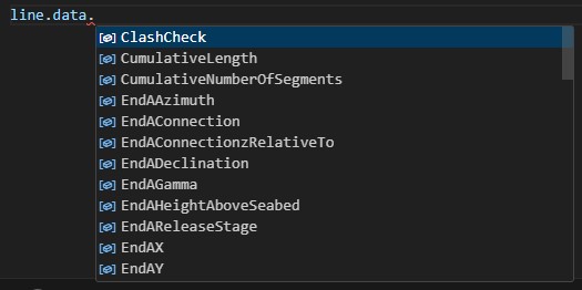
In addition, a hint shows the description of the parameter (mouse cursor stopped in the data name).
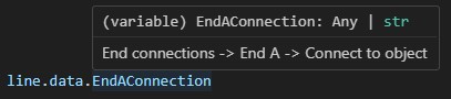
In the exemple below, data names of general, environment, and line objects are accessed
model.general.data.ImplicitConstantTimeStep = 0.01 # data from general object
model.environment.data.WaveHeight = 5.0 # data from environment object
line.data.EndAConnection = 'Anchored' # data form the line object
The line could be alse located by name with the following method. Although it could be done with the original method (line = model['Line1']), the new method is recommended to allow the functionality of auto-complete (data attribute)
line = model.findLineByName('Line1')
A list of all lines in the model may be retrieved and then select the first one by
lines = model.getAllLines()
line1 = lines[0]
Example 2 - Reduced simulation time for irregular wave
import NsgOrcFx as ofx
model = ofx.Model()
# set irregular wave
model.environment.data.WaveType = 'JONSWAP'
model.environment.data.WaveHs = 2.5
model.environment.data.WaveGamma = 2
model.environment.data.WaveTp = 8
# set reduced simulation duration with 200 seconds
model.SetReducedSimulationDuration(200)
# save data file to check the wave history
model.Save('reduced.dat')
# after executing this code, open the generated data file
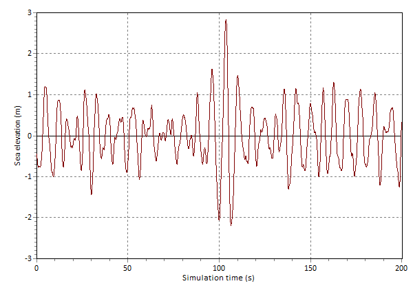
# then open Environment -> Waves preview, and set duration of 200s
# click in View profile and observe that the largest event (rise or fall)
# is in the midle of the sea elevation history
Example 3 - Generate load cases
import NsgOrcFx

model = NsgOrcFx.Model()
model.CreateLine()

# list of wave direction, height, and periods to define the Load Cases (LCs)
directions = [0, 45, 90]
heights = [1.5, 2.0, 3.0]
periods = [5, 7, 9]

# Folder to save the generated files (LCs)
outFolder = 'tmp'

# Regular waves
model.GenerateLoadCases('Dean stream', directions, heights, periods, outFolder)
In case of irregular wave:
model.GenerateLoadCases('JONSWAP', directions, heights, periods, outFolder)
To run irregular waves with reduced simulation time, based on the occurance of the largest rise or fall in the specified storm period.
model.GenerateLoadCases('JONSWAP', directions, heights, periods, outFolder, reducedIrregDuration=200)
Example 4 - Calculating modal analysis and getting the normalized modal shape
import NsgOrcFx

model = NsgOrcFx.Model()
model.CreateLine()

modes = model.CalculateModal()

# mode shape index (0 for the 1st)
modeIndex = 0

# mode frequency
freq = modes.getModeFrequency(modeIndex)

# if normalize = True, the displacements will be normalized, so the maximum total displacements is equal to the line diameter
[arcLengths, Ux, Uy, Uz] = modes.GlobalDispShape('Line1', modeIndex, True)
print('Frequency = ', freq, 'Hz')
print(arcLengths, Ux, Uy, Uz)
Example 5 - Defining fatigue analysis and getting the fatigue life calculated
import NsgOrcFx

simFile = r'tests\tmp\fatigue.sim'
ftgFile = r'tests\tmp\fatigue.ftg'

# First, it is necessary a model with simulation complete
model = NsgOrcFx.Model()
model.CreateLine()
model.RunSimulation()
model.Save(simFile)

# The fatigue analysis is defined, including the S-N curve based on the DNV-RP-C203
analysis = NsgOrcFx.FatigueAnalysis()
analysis.data.AnalysisType = 'Rainflow'
analysis.data.LoadCaseCount = 1
analysis.addLoadCase(simFile)
analysis.addSNCurveByNameAndEnv('F3','seawater')
analysis.addAnalysisData()
analysis.Calculate()
analysis.Save(ftgFile)

# Result of fatigue life in each node
lifePerNode = analysis.getLifeList()
print(lifePerNode)
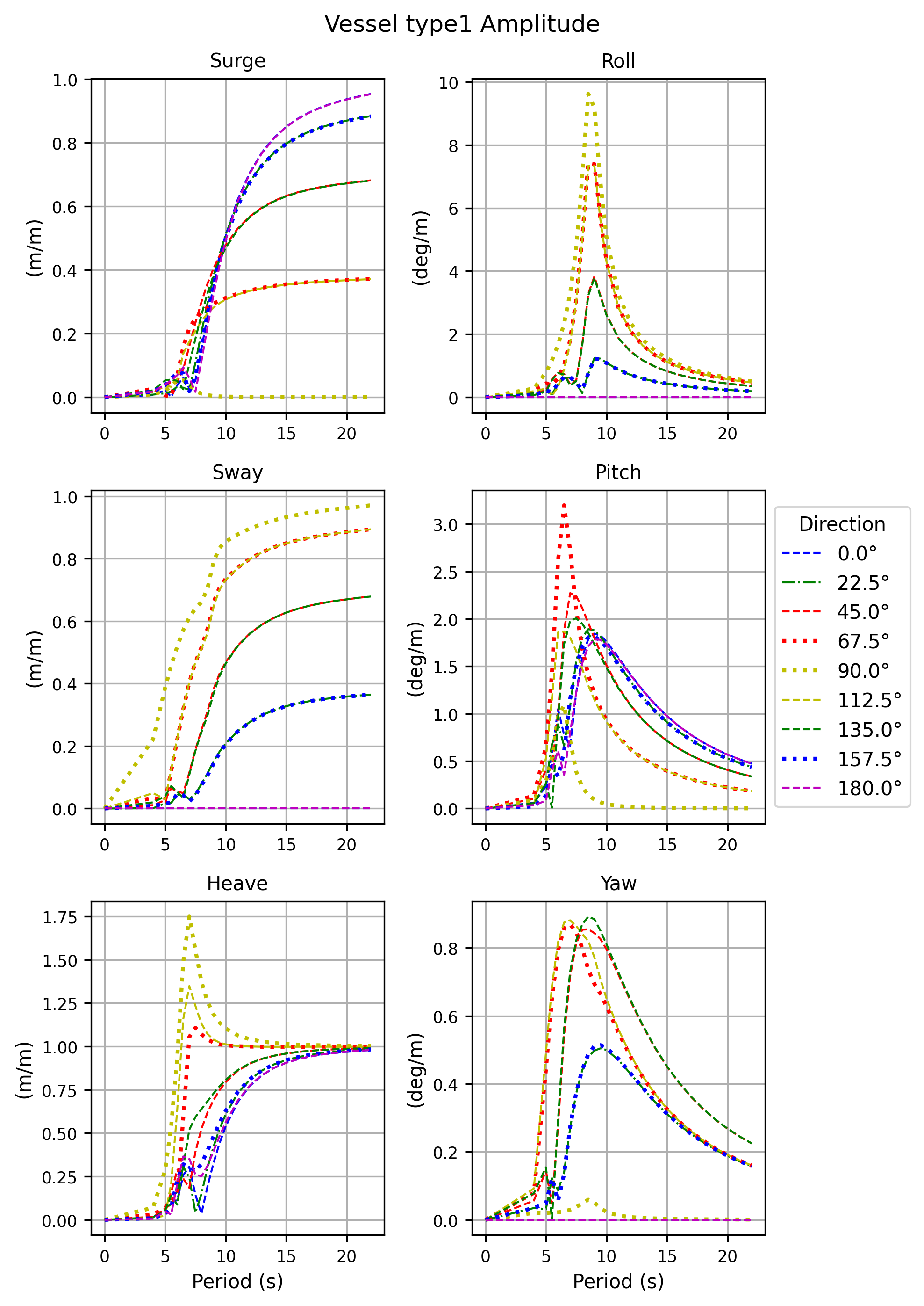
Example 6 - Generates RAO plots from vessel type data
import NsgOrcFx as ofx

model = ofx.Model()

# Create a 'Vessel Type' object with default data
model.CreateObject(ofx.ObjectType.VesselType)

# Create RAO plots (amplitude and phase) and save to the defined folder
model.SaveRAOplots(r'tests\tmptestfiles')
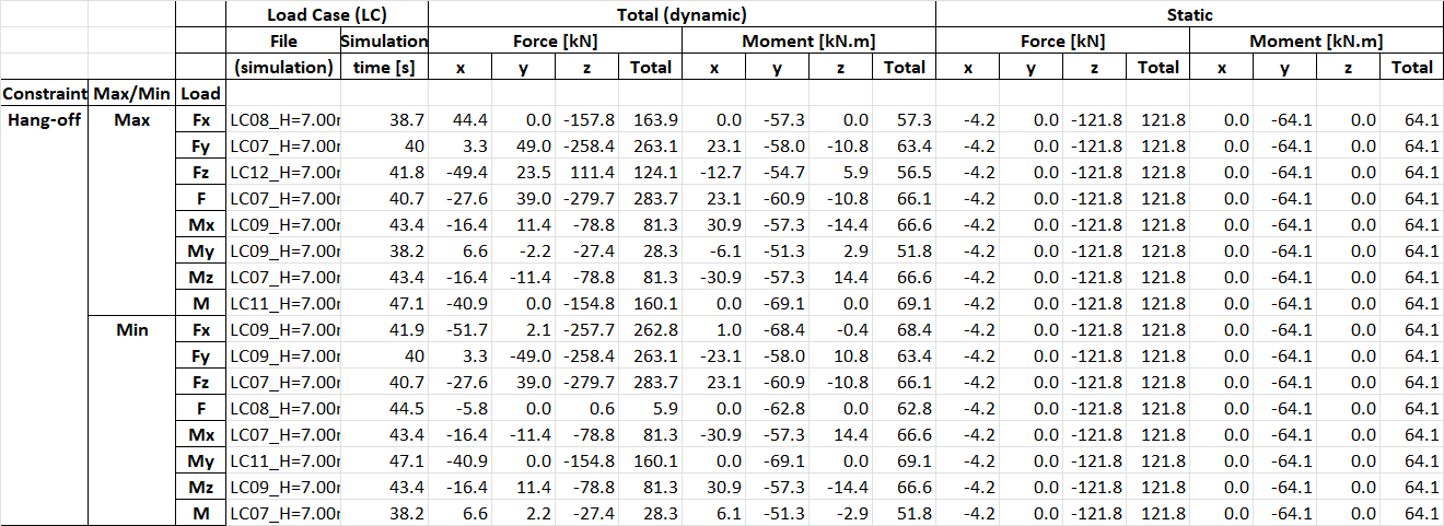
Example 7 - Extract extreme (max. and min.) Constraint loads (force and moment) from multiple simulation files
import NsgOrcFx as ofx

model = ofx.Model()

# create the objects (vessel, constraint, and line)
vessel = model.CreateObject(ofx.ObjectType.Vessel)
constraint = model.CreateObject(ofx.ObjectType.Constraint)
line = model.CreateObject(ofx.ObjectType.Line)

# connect the constraint to the vessel
constraint.name = 'Hang-off'
constraint.InFrameConnection = vessel.name
constraint.InFrameInitialX = 35
constraint.InFrameInitialY = 0
constraint.InFrameInitialZ = -7
constraint.InFrameInitialDeclination = 155 # adjust the nominal top angle

# connect the line End A to the constraint,
# anchor the End B, 155m horizontally away from A,
# and set the line length
line.EndAConnection = constraint.name
line.EndAX, line.EndAY, line.EndAZ = 0, 0, 0
line.EndAxBendingStiffness = ofx.OrcinaInfinity() # to produce moment reaction loads to extract
line.EndBConnection = 'Anchored'
line.PolarReferenceAxes[1] = 'Global Axes'
line.PolarR[1], line.EndBY, line.EndBHeightAboveSeabed = 155, 0, 0
line.Length[0] = 200

# generate the load cases (Example #3)
model.GenerateLoadCases('Dean stream', [135,180,225], [6,7], [9,10], '.')

# run the simulations with multi-threading
ofx.ProcMultiThread('.','.')

# extract extreme loads for the constraint
ofx.ExtremeLoadsFromConstraints('.','.\Results.xlsx')
Release history Release notifications | RSS feed


Download files
Download the file for your platform. If you're not sure which to choose, learn more about installing packages.
Source Distribution
Built Distribution
Filter files by name, interpreter, ABI, and platform.
If you're not sure about the file name format, learn more about wheel file names.
Copy a direct link to the current filters
File details
Details for the file nsgorcfx-1.0.34.tar.gz.
File metadata
- Download URL: nsgorcfx-1.0.34.tar.gz
- Upload date:
- Size: 43.9 kB
- Tags: Source
- Uploaded using Trusted Publishing? No
- Uploaded via: twine/6.2.0 CPython/3.12.0
File hashes
| Algorithm | Hash digest | |
|---|---|---|
| SHA256 |
fecf187811f2b7b2dd1913d15c768443d8e2d94504e182fe74b85282214ad8fa
|
|
| MD5 |
04fc7dfc55c1a5f56df1f7ca1e0ceadb
|
|
| BLAKE2b-256 |
a9267b5e947371597d404c743f328baa7248eba635953b0a7ecff8a1b8a08d8e
|
File details
Details for the file nsgorcfx-1.0.34-py3-none-any.whl.
File metadata
- Download URL: nsgorcfx-1.0.34-py3-none-any.whl
- Upload date:
- Size: 48.1 kB
- Tags: Python 3
- Uploaded using Trusted Publishing? No
- Uploaded via: twine/6.2.0 CPython/3.12.0
File hashes
| Algorithm | Hash digest | |
|---|---|---|
| SHA256 |
bd9a8fbc81eaa6ed1ff0b01ee3340e33ce85473c62875fadc3b7f8df3aa205ae
|
|
| MD5 |
6a6b72352727a49260620c95f258d7bb
|
|
| BLAKE2b-256 |
ab1e8def6303898e9c582aa370227c4be07e30e1212dcdbda2a65d04dc0d2cae
|


