Geomagnetic Cutoff Computation Tool

Project description

OTSOpy
Python package version of the OTSO tool used for trajectory computations of charged particles in the Earth's magnetosphere.
OTSO is designed to be open-source; all suggestions for improvement are welcome, and please report any bugs you find. I welcome any help provided by the community in the development of OTSO.
Disclaimer! OTSOpy is currently only available for Python 3.12. This is due to the compiled Fortran libraries being Python version-specific. It is recommended that you set up a new Python environment using Python 3.12. Users may attempt to clone the repository and compile the Fortran code themselves with f2py, following instructions on the original OTSO repository. I will attempt to keep OTSOpy compatible with as many Python versions as possible. However, I hope that the open-source nature of the OTSO tool means that the compiled Fortran libraries users make will be shared and merged with this release, relieving me of some of the pressure.
Installation
Installation of OTSOpy is designed to be as simple as possible and can be done utilising pip. Users have two options when downloading OTSOpy.
Option 1: PyPi
Users may install OTSO directly from PyPi using:
pip install OTSO
This will install OTSO into your current Python environment.
Option 2: Repository
Users may clone the repository and run the setup.py file within the main OTSOpy directory using:
pip install .
This will install OTSO into your current Python environment.
Functions
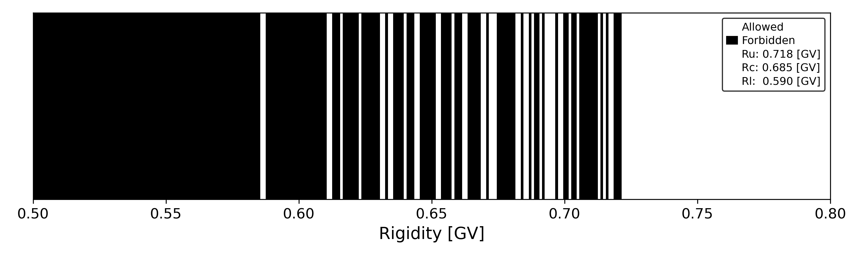
Cutoff
Computes the geomagnetic cut-off rigidities for given locations around the Earth under user-inputted geomagnetic conditions.
Cone
Computes the asymptotic viewing directions for given locations around the Earth. Asymptotic latitudes and longitudes over a range of rigidity values are computed. Asymptotic latitude and longitude can be given in any available coordinate system.
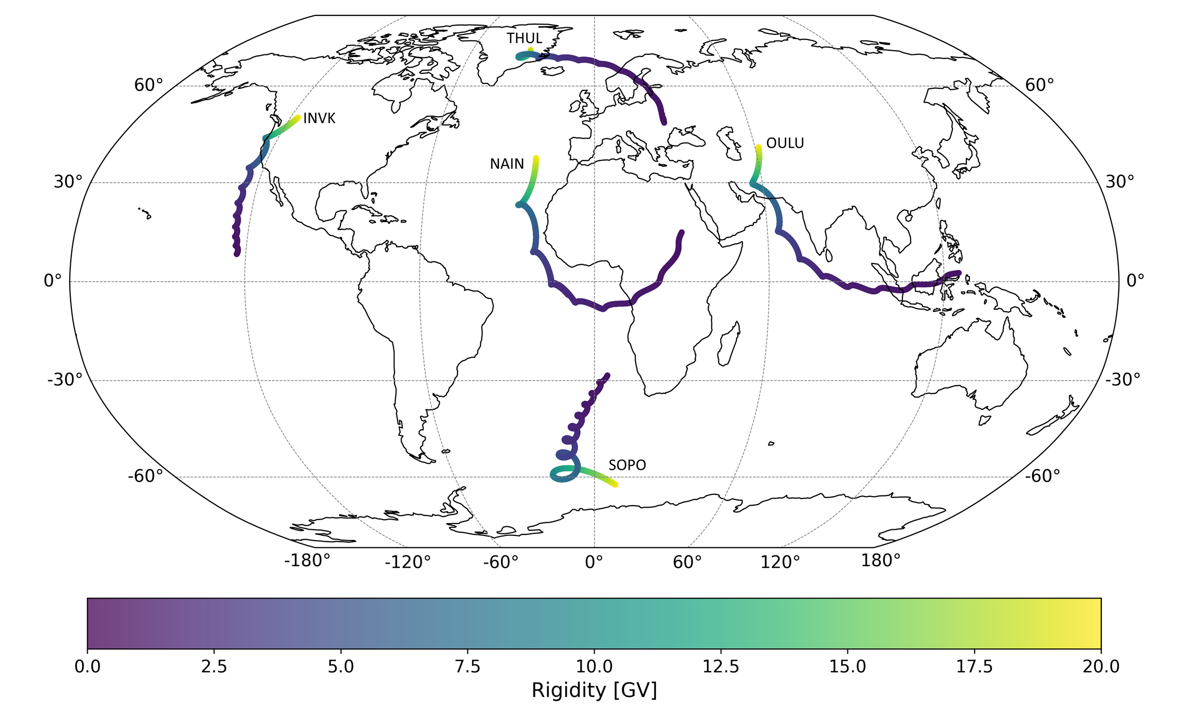
Figure 2: Asymptotic cones for the Oulu, Nain, South Pole, Thule, and Inuvik neutron monitors for the IGRF 2010 epoch and TSY89 model, with kp = 0. Latitudes and longitudes are in the geocentric coordinate system.
Trajectory
Computes and outputs the trajectory of a charged particle with a specified rigidity from a given start location on Earth. Positional information can be in any of the available coordinate systems.
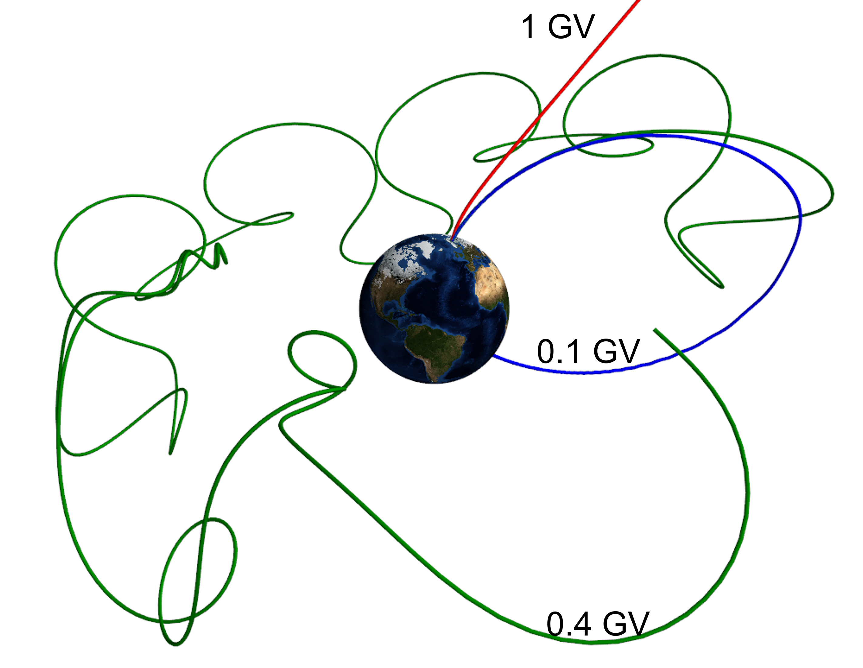
Figure 3: Computed trajectories of three cosmic rays of various rigidity values being backtraced from the Oulu neutron monitor for the IGRF 2000 and TSY89 model, with kp = 0. The 1GV particle is allowed (able to escape the magnetosphere); the 0.4GV particle is forbidden (it is trapped in the magnetosphere); and the 0.1GV is also forbidden (it returns to Earth).
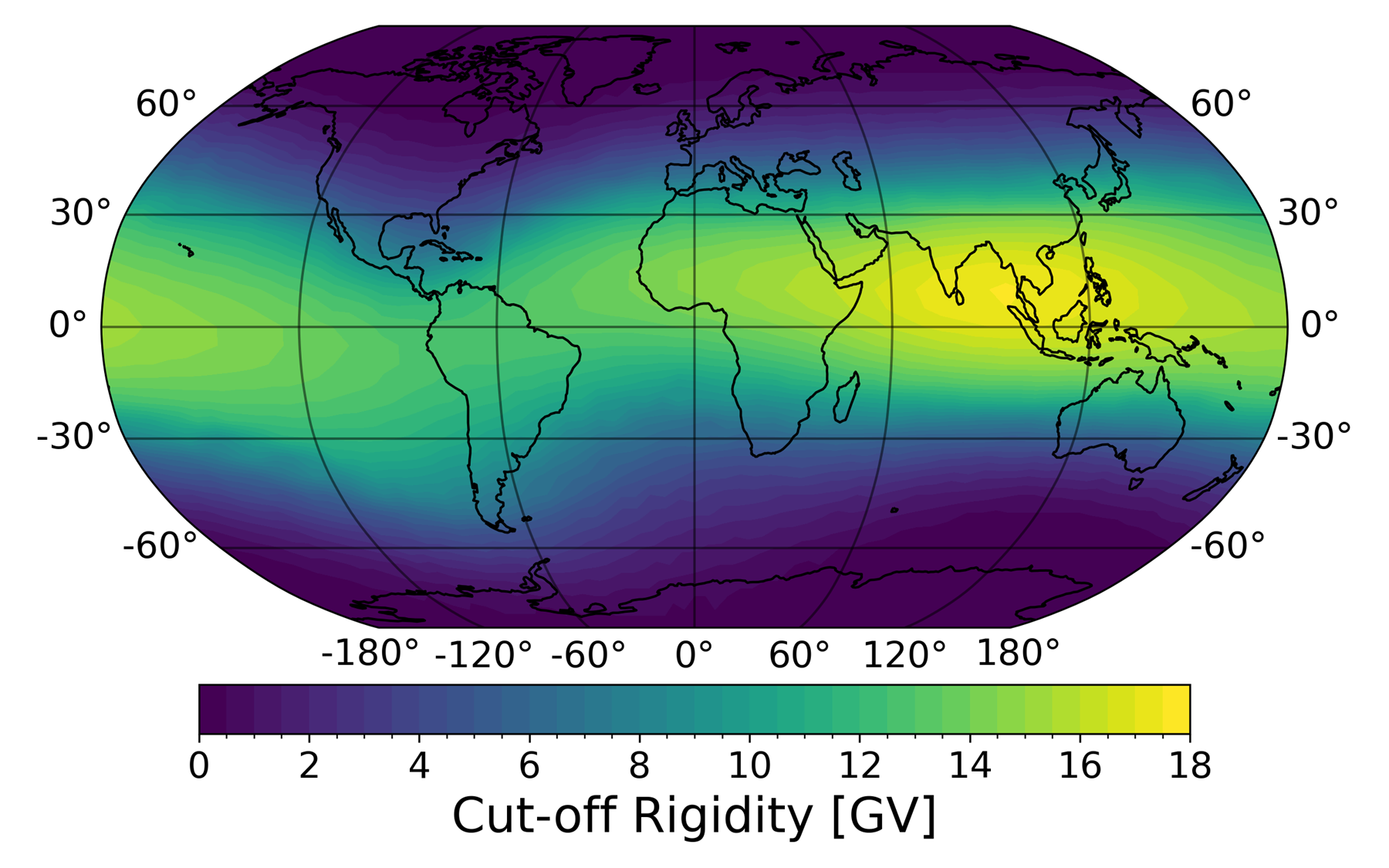
Planet
Performs the cutoff function over a user-defined location grid, allowing for cutoffs for the entire globe to be computed instead of individual locations. There is the option to return the asymptotic viewing directions at each computed location by utilising a user-inputted list of rigidity levels.
Flight
Computes the cut-off rigidities along a user-defined path. The function is named Flight as it is primarily been developed for use in aviation tools, but any path can be entered. For example, the function can be applied to geomagnetic latitude surveys using positional data from a ship voyage, or it can be used to compute anisotropy and cut-off values for low-Earth orbit spacecraft. This function allows for changing altitude, location, and date values.
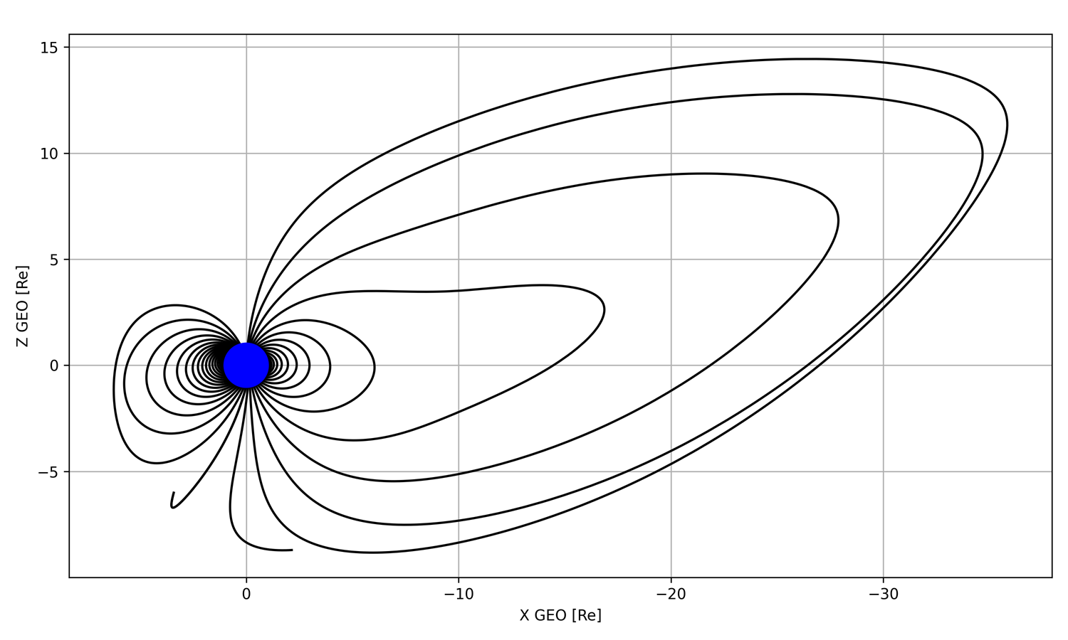
Trace
Traces the magnetic field lines around the globe or for a given location based on the geomagnetic configuration detailed by the user. It is useful for modelling the magnetosphere structure under disturbed conditions and for finding open magnetic field lines.
Coordtrans
Converts input positional information from one coordinate system to another, utilising the IRBEM library of coordinate transforms.
Magfield
Computes the total magnetic field strength at a given location depending on the user's input geomagnetic conditions. Outputs will be in the geocentric solar magnetospheric (GSM) coordinate system.
Examples
Cutoff
import OTSO

if __name__ == '__main__':
    stations_list = ["OULU", "ROME", "ATHN", "CALG"]  # list of neutron monitor stations (using their abbreviations)

    cutoff = OTSO.cutoff(Stations=stations_list, corenum=1, year=2000, month=1, day=1, hour=0)

    print(cutoff[0])  # dataframe output containing Ru, Rc, Rl for all input locations
    print(cutoff[1])  # text output of input variable information
Output
Ru = upper cut-off rigidity [GV]
Rc = effective cut-off rigidity [GV]
Rl = lower cut-off rigidity [GV]
      ATHN  CALG  OULU  ROME
Ru    8.92  1.15  0.72  6.34
Rc    8.68  1.12  0.67  6.17
Rl    8.57  1.02  0.62  5.00
Cone
import OTSO

if __name__ == '__main__':

    stations_list = ["OULU","ROME","ATHN","CALG"] # list of neutron monitor stations (using their abbreviations)

    cone = OTSO.cone(Stations=stations_list,corenum=1,year=2000,month=1,day=1,hour=0)

    print(cone[0]) # dataframe output containing asymptotic cones for all input locations
    print(cone[1]) # dataframe output containing Ru, Rc, Rl for all inputted locations
    print(cone[2]) # text output of input variable information
Output
Showing only the cone[0] output containing the asymptotic viewing directions of the input stations. Result layout is: filter;latitude;longitude. If the filter value is 1, then the particle of that rigidity has an allowed trajectory. If the filter value is NOT 1, then the particle of that rigidity has a forbidden trajectory.
      R [GV]                ATHN              CALG               OULU                ROME
0     20.000     1;-1.599;89.139  1;21.147;271.981    1;40.892;62.428      1;4.077;71.061
1     19.990     1;-1.625;89.166  1;21.132;271.980    1;40.879;62.427      1;4.052;71.080
2     19.980     1;-1.652;89.195  1;21.117;271.978    1;40.867;62.425      1;4.026;71.098
3     19.970     1;-1.678;89.222  1;21.102;271.976    1;40.854;62.424      1;4.000;71.117
4     19.960     1;-1.704;89.251  1;21.087;271.975    1;40.842;62.422      1;3.975;71.135
...      ...                 ...               ...                ...                 ...
1995   0.050   -1;18.921;202.260  -1;55.778;67.804  -1;43.146;232.544  -1;-23.689;191.552
1996   0.040  -1;-12.213;230.889  -1;31.434;54.166  -1;28.819;225.953    -1;5.443;168.553
1997   0.030   -1;15.332;187.614  -1;57.549;27.604  -1;28.198;224.400   -1;22.447;205.148
1998   0.020   -1;18.778;204.219  -1;50.931;22.612  -1;25.831;217.207   -1;12.262;170.688
1999   0.010   -1;-6.034;230.324  -1;30.431;41.536  -1;36.856;197.770   -1;24.229;184.606
Trajectory
import OTSO

if __name__ == '__main__':

    stations_list = ["OULU","ROME","ATHN","CALG"] # list of neutron monitor stations (using their abbreviations)

    trajectory = OTSO.trajectory(Stations=stations_list,rigidity=5,corenum=1)

    print(trajectory[0]) # dictionary output containing positional information for all trajectories generated starting
                         # from input stations
    print(trajectory[1]) # text output of input variable information
Output
Showing the dataframe produced for the particle originating from Oulu. Other trajectories are within the trajectory[0] dictionary.
'OULU':
       X_Re [GEO]  Y_Re [GEO]  Z_Re [GEO]
0      0.383681    0.182761    0.907372
1      0.383888    0.182861    0.907864
2      0.384114    0.182973    0.908405
3      0.384363    0.183098    0.909000
4      0.384636    0.183238    0.909654
..          ...         ...         ...
218    6.759500    9.079110    5.098440
219    6.762920    9.085720    5.100750
220    6.766340    9.092320    5.103050
221    6.769770    9.098930    5.105360
222    6.773190    9.105540    5.107660
Planet
import OTSO

if __name__ == '__main__':

    planet = OTSO.planet(corenum=1, cutoff_comp="Vertical", year=2000, rigiditystep=0.1)

    print(planet[0]) # dataframe containing cutoff results for planet grid
    print(planet[1]) # text output of input variable information
Output
The default output is a 5°x5° grid of the Earth with no asymptotic viewing directions computed.
      Latitude  Longitude   Rl   Rc   Ru
0        -90.0        0.0  0.0  0.0  0.0
1        -90.0        5.0  0.0  0.0  0.0
2        -90.0       10.0  0.0  0.0  0.0
3        -90.0       15.0  0.0  0.0  0.0
4        -90.0       20.0  0.0  0.0  0.0
...        ...        ...  ...  ...  ...
2696      90.0      340.0  0.0  0.0  0.0
2697      90.0      345.0  0.0  0.0  0.0
2698      90.0      350.0  0.0  0.0  0.0
2699      90.0      355.0  0.0  0.0  0.0
2700      90.0      360.0  0.0  0.0  0.0
Flight
import OTSO
import datetime

if __name__ == '__main__':

    latitude_list = [10,15,20,25,30] # [Latitudes]
    longitude_list = [10,15,20,25,30] # [Longitudes]
    altitude_list = [30,40,50,60,80] # [Altitudes] in km
    date_list = [datetime.datetime(2000,10,12,8),datetime.datetime(2000,10,12,9),datetime.datetime(2000,10,12,10),
                 datetime.datetime(2000,10,12,11),datetime.datetime(2000,10,12,12)] # [dates]


    flight = OTSO.flight(latitudes=latitude_list, longitudes=longitude_list,dates=date_list,
                         altitudes=altitude_list,cutoff_comp="Vertical",corenum=1)

    print(flight[0]) # dataframe output containing Ru, Rc, Rl along flightpath
    print(flight[1]) # text output of input variable information
    print(flight[2]) # dataframe output of input variables
Output
flight[0] dataframe output.
                  Date  Latitude  Longitude  Altitude     Ru     Rc     Rl
0  2000-10-12 08:00:00        10         10        30  14.86  14.86  14.86
1  2000-10-12 09:00:00        15         15        40  14.90  14.90  14.90
2  2000-10-12 10:00:00        20         20        50  14.48  14.48  14.48
3  2000-10-12 11:00:00        25         25        60  13.59  13.59  13.59
4  2000-10-12 12:00:00        30         30        80  12.18  11.49  10.39
Trace
import OTSO

if __name__ == '__main__':

    trace = OTSO.trace(corenum=1)

    print(trace[0]) # dictionary output containing positional information of magnetic field lines generated over
                    # the globe
    print(trace[1]) # text output of input variable information
Output
Example output of one of the field line traces for the location latitude = 10° and longitude = 355°.
'10_355':
      X_GEO [Re]  Y_GEO [Re]  Z_GEO [Re]  Bx_GSM [nT]  By_GSM [nT]  Bz_GSM [nT]
0     0.985162   -0.086269    0.174797    -0.000015     0.000003     0.000028
1     0.985008   -0.086334    0.176358    -0.000015     0.000003     0.000028
2     0.984845   -0.086397    0.177918    -0.000016     0.000003     0.000028
3     0.984673   -0.086459    0.179477    -0.000016     0.000003     0.000028
4     0.984493   -0.086521    0.181035    -0.000016     0.000003     0.000028
..         ...         ...         ...          ...          ...          ...
56    0.963476   -0.088020    0.259596    -0.000024     0.000004     0.000023
57    0.962858   -0.088017    0.261038    -0.000024     0.000004     0.000023
58    0.962232   -0.088012    0.262478    -0.000025     0.000004     0.000023
59    0.961599   -0.088007    0.263914    -0.000025     0.000004     0.000023
60    0.960958   -0.088000    0.265346    -0.000025     0.000004     0.000023
Coordtrans
import OTSO
import datetime

if __name__ == '__main__':

    lat_lon_alt_list = [[10,10,10]] # [[Latitude,Longitude,Altitude]]
    date_list = [datetime.datetime(2000,10,12,8)] # [dates]

    Coords = OTSO.coordtrans(Locations=lat_lon_alt_list,Dates=date_list,CoordIN="GEO",CoordOUT="GSM",corenum=1)

    print(Coords[0]) # dataframe output of converted coordinates
    print(Coords[1]) # text output detailing the initial and final conversion coordinate system
Output
Coords[0] output converting the [10,10,10] position from GEO coordinate system to GSM coordinate system.
                  Date X_GEO [Re] Y_GEO [Re] Z_GEO [Re] X_GSM [Re] Y_GSM [Re] Z_GSM [Re]
0  2000-10-12 08:00:00    1.00157       10.0       10.0   7.508443   6.239805  10.280626
Magfield
import OTSO

if __name__ == '__main__':

    location_list = [[10,10,10]] # [[X,Y,Z]] Earth radii Geocentric coordinates in this instance

    magfield = OTSO.magfield(Locations=location_list,coordsystem="GEO",corenum=1)

    print(magfield[0]) # dataframe of returned magnetic field vectors at input locations
    print(magfield[1]) # text output of input variable information
Output
magfield[0] output showing the magnetic field vector at the input location in the GSM coordinate system.
   X_GEO [Re]  Y_GEO [Re]  Z_GEO [Re]  GSM_Bx [nT]  GSM_By [nT]  GSM_Bz [nT]
0        10.0        10.0        10.0    10.735511    -2.413911    11.586166
Acknowledgements
The fantastic IRBEM library has been used in the development of OTSO, which proved an invaluable asset and greatly sped up development. The latest release of the IRBEM library can be found at https://doi.org/10.5281/zenodo.6867552. Thank you to N. Tsyganenko for the development of the external magnetic field models and their code, which are used within OTSO.
A wider thanks goes to the space physics community who, through the use of the original OTSO, provided invaluable feedback, advice on improvements, and bug reporting. All discussions and advice have aided in the continual development and improvement of OTSO, allowing it to fulfil its aim of being a community-driven open-source tool. The lessons learned from the initial OTSO versions have been incorporated into OTSOpy. Dr. Chris Davis was also instrumental in the development of OTSOpy with his suggestion of incorporating OTSO into the AniMARIE tool, initiating the package development and providing help by expanding functionality and bug fixing. OTSO was developed at the University of Oulu as part of the Academy of Finland QUASARE project. I would like to thank my colleagues at the University and the Academy of Finland for supporting the work.
References
- Larsen, N., Mishev, A., & Usoskin, I. (2023). A new open-source geomagnetosphere propagation tool (OTSO) and its applications. Journal of Geophysical Research: Space Physics, 128, e2022JA031061. https://doi.org/10.1029/2022JA031061
Release history Release notifications | RSS feed


Download files
Download the file for your platform. If you're not sure which to choose, learn more about installing packages.
Source Distribution
Built Distribution
Filter files by name, interpreter, ABI, and platform.
If you're not sure about the file name format, learn more about wheel file names.
Copy a direct link to the current filters
File details
Details for the file otso-1.0.10.tar.gz.
File metadata
- Download URL: otso-1.0.10.tar.gz
- Upload date:
- Size: 4.8 MB
- Tags: Source
- Uploaded using Trusted Publishing? No
- Uploaded via: twine/6.1.0 CPython/3.12.10
File hashes
| Algorithm | Hash digest | |
|---|---|---|
| SHA256 |
f19e1ed2294ac08942207b3d481ca38139a6def2af3675c4ef35d78542844f8d
|
|
| MD5 |
e8b231920578f9ce290f9f966200c4b6
|
|
| BLAKE2b-256 |
bad295f0d2c716169f288581176c0a94851f233c5580d50b4aedd5dc6fee895b
|
File details
Details for the file otso-1.0.10-py3-none-any.whl.
File metadata
- Download URL: otso-1.0.10-py3-none-any.whl
- Upload date:
- Size: 4.9 MB
- Tags: Python 3
- Uploaded using Trusted Publishing? No
- Uploaded via: twine/6.1.0 CPython/3.12.10
File hashes
| Algorithm | Hash digest | |
|---|---|---|
| SHA256 |
2936a4c39173f031fd94d71cf208d7a8969f93efe793ff7bf5860fc0b987dcc6
|
|
| MD5 |
7621220606a75b95fe657934c834c2f5
|
|
| BLAKE2b-256 |
a2dfd85da40557d863379d80f6a8f997678937e6ee9b0bd2a056e6803eca5629
|


