Octave-Band and Fractional Octave-Band filter for signals in time domain.

Project description


PyOctaveBand
Advanced Octave-Band and Fractional Octave-Band filter bank for signals in the time domain. Fully compliant with ANSI s1.11-2004 and IEC 61260-1-2014.
This library provides professional-grade tools for acoustic analysis, including frequency weighting (A, C, Z), time ballistics (Fast, Slow, Impulse), and multiple filter architectures.
Now available on PyPI.
📑 Table of Contents
- 🚀 Getting Started
- 🛠️ Filter Architectures
- 🔊 Acoustic Weighting (A, C, Z)
- ⏱️ Time Weighting and Integration
- ⚡ Performance: OctaveFilterBank
- 🔍 Filter Usage and Examples
- 📏 Calibration and dBFS
- 📊 Signal Decomposition
- 📖 Theory and Equations
- 🧪 Testing and Quality
🚀 Getting Started
Installation
Option 1: From PyPI (Recommended)
Install PyOctaveBand directly using pip:
pip install PyOctaveBand
Option 2: Cloning and Installing Clone the repository and install it manually:
git clone https://github.com/jmrplens/PyOctaveBand.git
cd PyOctaveBand
pip install .
Option 3: Git Submodule
Add PyOctaveBand as a dependency within your own git repository:
git submodule add https://github.com/jmrplens/PyOctaveBand.git
# Then install in editable mode to use it from your project
pip install -e ./PyOctaveBand
Basic Usage: 1/3 Octave Analysis
Analyze a signal and get the Sound Pressure Level (SPL) per frequency band.
import numpy as np
from pyoctaveband import octavefilter

fs = 48000
t = np.linspace(0, 1, fs)
# Composite signal: 100Hz + 1000Hz
signal = np.sin(2 * np.pi * 100 * t) + np.sin(2 * np.pi * 1000 * t)

# Apply 1/3 octave filter bank
spl, freq = octavefilter(signal, fs=fs, fraction=3)

print(f"Bands: {freq}")
print(f"SPL [dB]: {spl}")
🛠️ Filter Architectures
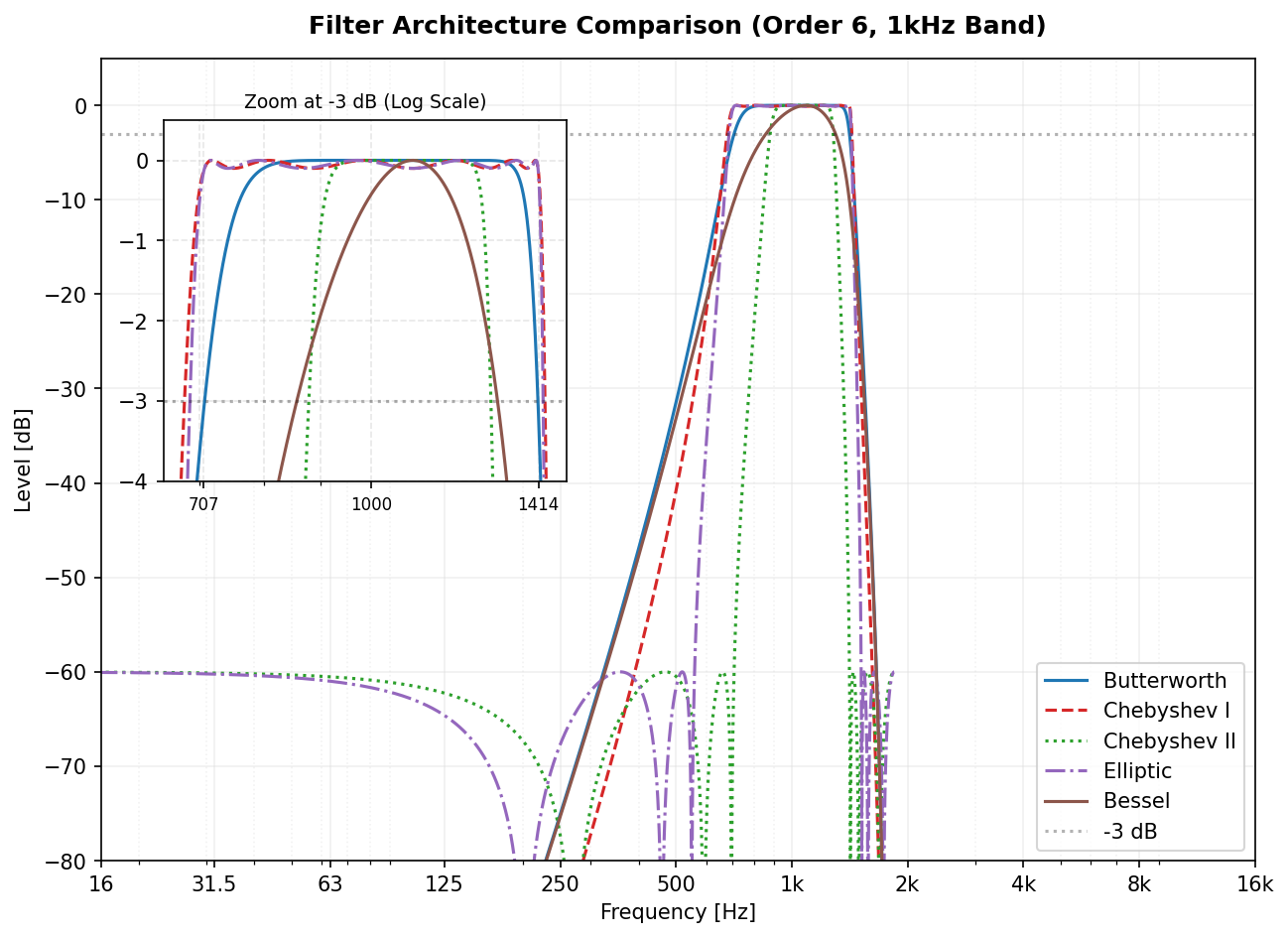
PyOctaveBand supports several filter types, each with its own transfer function characteristic.
Filter Comparison and Zoom
We use Second-Order Sections (SOS) for all filters to ensure numerical stability. The following plot compares the architectures focusing on the -3 dB crossover point.
| Type | Name | Usage Example | Best For |
|---|---|---|---|
butter |
Butterworth | octavefilter(x, fs, filter_type='butter') |
General acoustic measurement. |
cheby1 |
Chebyshev I | octavefilter(x, fs, filter_type='cheby1', ripple=0.1) |
Sharper roll-off at the cost of ripple. |
cheby2 |
Chebyshev II | octavefilter(x, fs, filter_type='cheby2', attenuation=60) |
Flat passband with stopband zeros. |
ellip |
Elliptic | octavefilter(x, fs, filter_type='ellip', ripple=0.1, attenuation=60) |
Maximum selectivity. |
bessel |
Bessel | octavefilter(x, fs, filter_type='bessel') |
Preserving transient waveform shapes. |
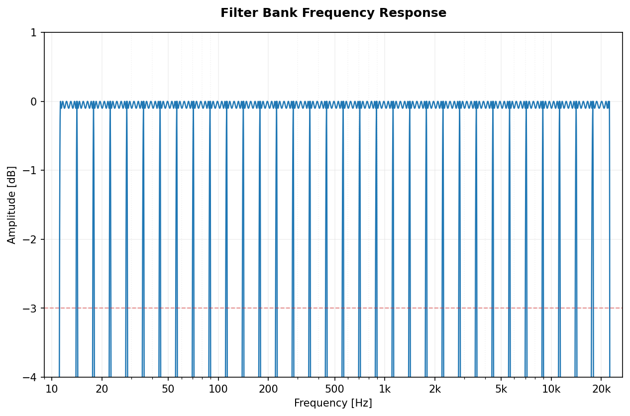
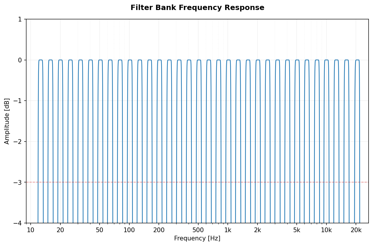
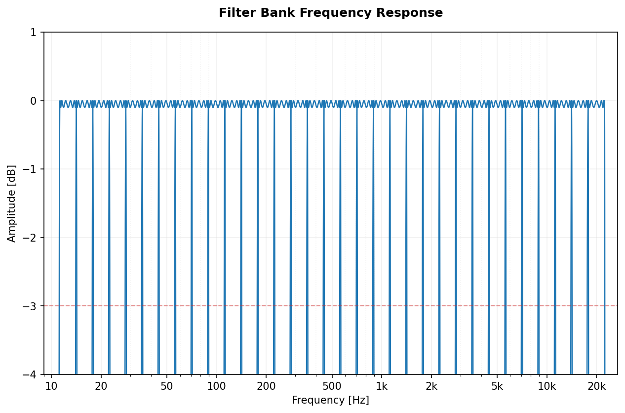
Gallery of Filter Bank Responses
Full spectral view of the filter banks for Octave (1/1) and 1/3-Octave fractions.
| Architecture | 1/1 Octave (Fraction=1) | 1/3 Octave (Fraction=3) |
|---|---|---|
| Butterworth | 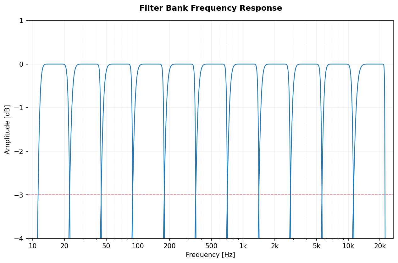 |
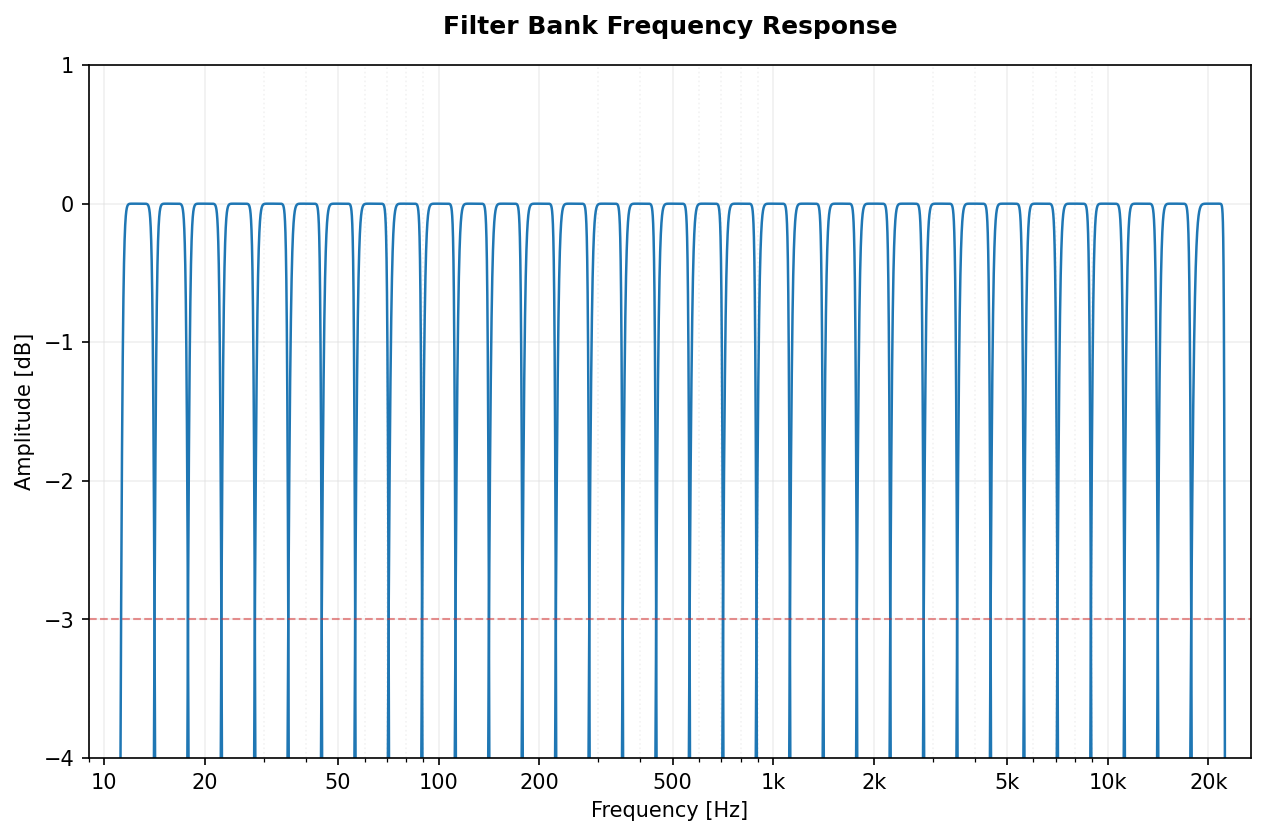 |
| Chebyshev I | 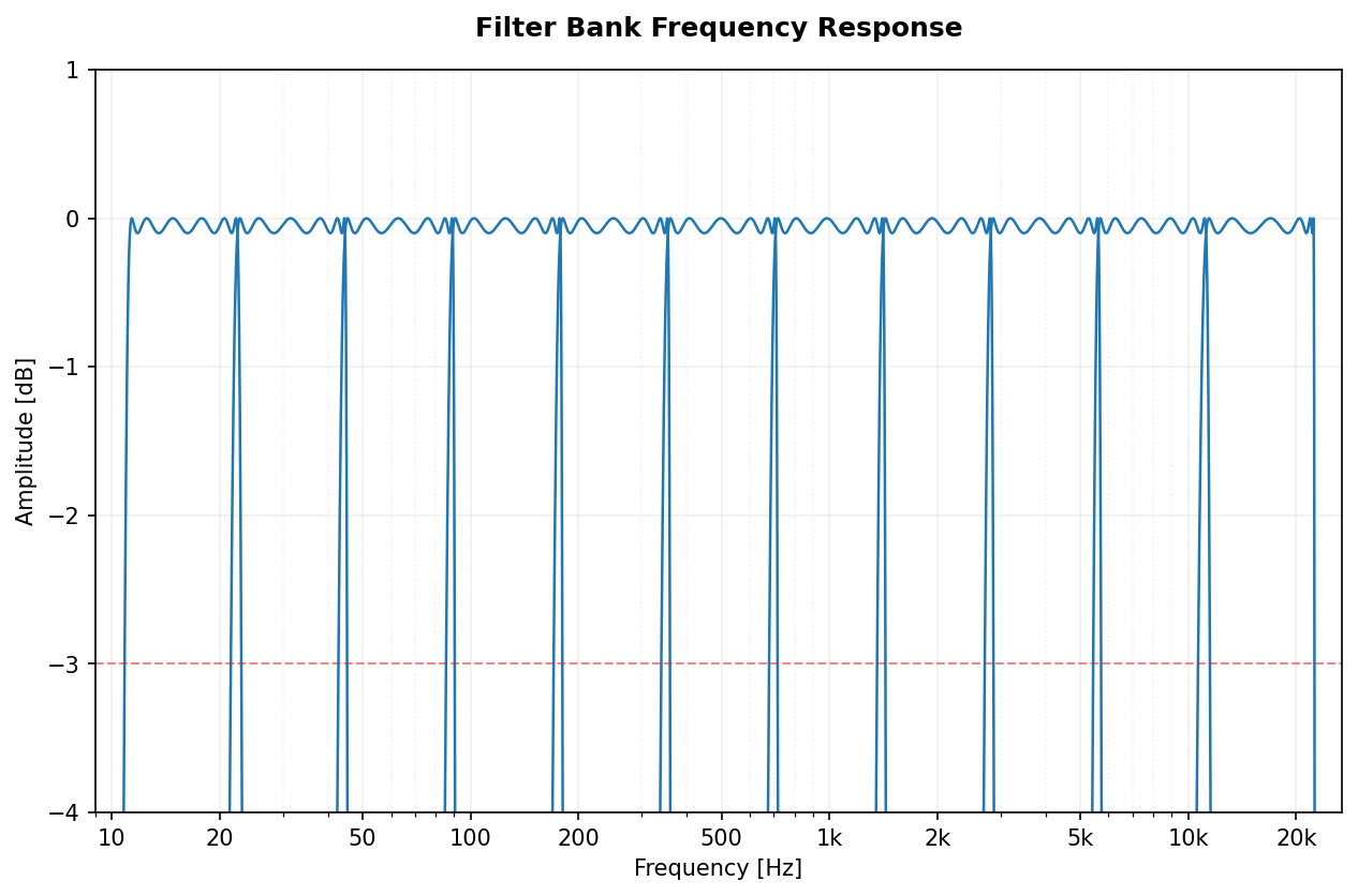 |
 |
| Chebyshev II | 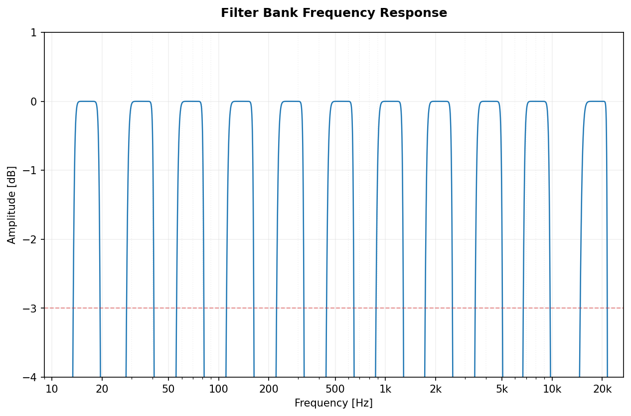 |
 |
| Elliptic |  |
 |
| Bessel | 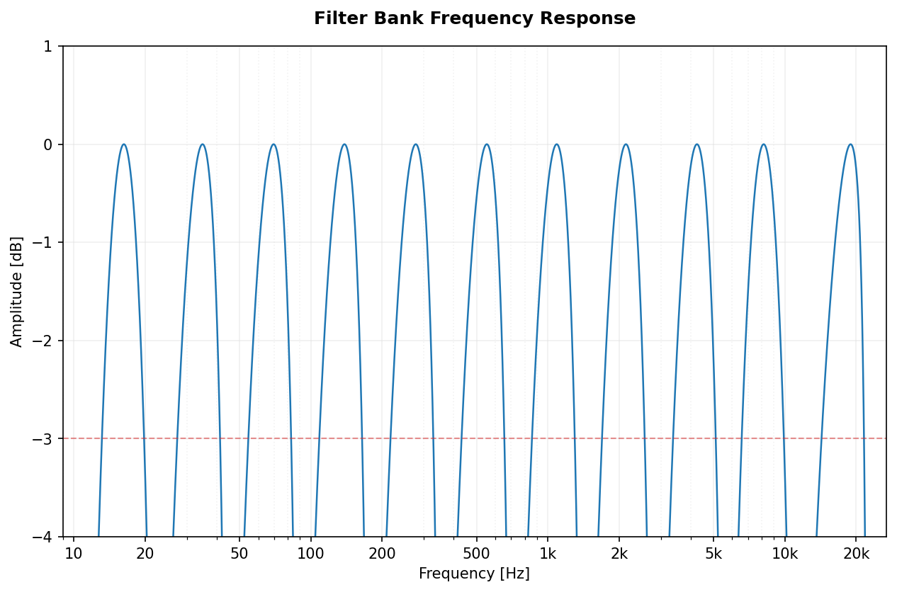 |
 |
🔊 Acoustic Weighting (A, C, Z)
Frequency weighting curves simulate the human ear's sensitivity.
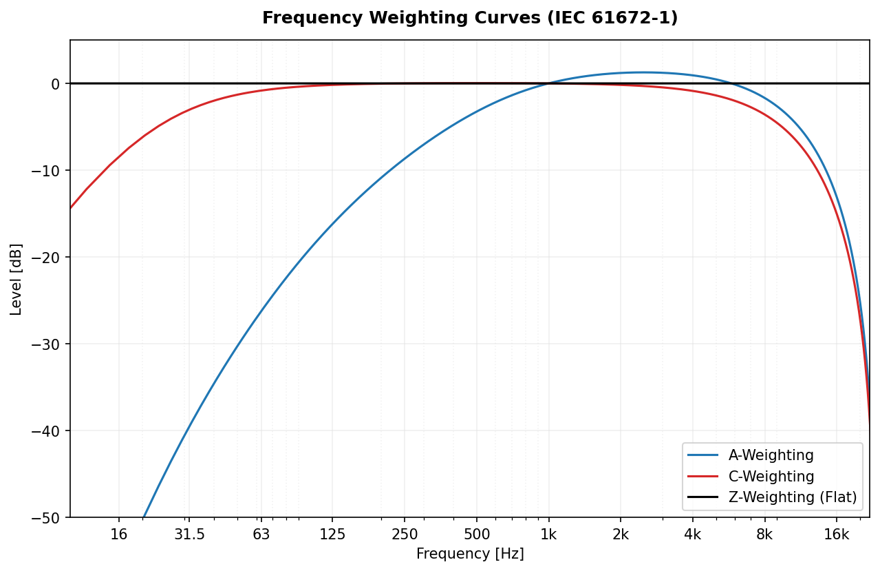
- A-Weighting (
A): Standard for environmental noise (IEC 61672-1). - C-Weighting (
C): Used for peak sound pressure and high-level noise. - Z-Weighting (
Z): Zero weighting, completely flat response.
from pyoctaveband import weighting_filter

# Apply A-weighting to the raw signal
weighted_signal = weighting_filter(signal, fs, curve='A')

# Apply C-weighting for peak analysis
c_weighted_signal = weighting_filter(signal, fs, curve='C')
⏱️ Time Weighting and Integration
Accurate SPL measurement requires capturing energy over specific time windows.
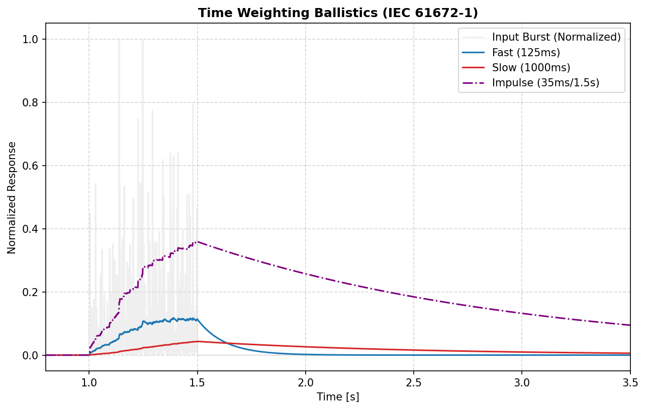
- Fast (
fast): $\tau = 125$ ms. Standard for noise fluctuations. - Slow (
slow): $\tau = 1000$ ms. Standard for steady noise. - Impulse (
impulse): 35 ms rise time. For explosive sounds.
from pyoctaveband import time_weighting

# Calculate energy envelope (Mean Square)
energy_envelope = time_weighting(signal, fs, mode='fast')
# dB SPL relative to 20μPa
spl_t = 10 * np.log10(energy_envelope / (2e-5)**2)
⚡ Performance: OctaveFilterBank Class
Pre-calculating coefficients saves significant CPU time when processing multiple frames.
from pyoctaveband import OctaveFilterBank

bank = OctaveFilterBank(fs=48000, fraction=3, filter_type='butter')

# Process multiple signals efficiently
for frame in stream:
    spl, freq = bank.filter(frame)
🔍 Filter Usage and Examples
This section provides detailed examples and characteristics for each supported filter architecture.
1. Butterworth (butter)
The Butterworth filter is known for its maximally flat passband. It is the standard choice for acoustic measurements where no ripple is allowed within the frequency bands.
from pyoctaveband import octavefilter
# Default standard measurement
spl, freq = octavefilter(x, fs, filter_type='butter')
2. Chebyshev I (cheby1)
Chebyshev Type I filters provide a steeper roll-off than Butterworth at the expense of ripples in the passband. Useful when high selectivity is needed near the cut-off frequencies.
# Selectivity with 0.1 dB passband ripple
spl, freq = octavefilter(x, fs, filter_type='cheby1', ripple=0.1)
3. Chebyshev II (cheby2)
Also known as Inverse Chebyshev, it has a flat passband and ripples in the stopband. It provides faster roll-off than Butterworth without affecting the signal in the passband.
# Flat passband with 60 dB stopband attenuation
spl, freq = octavefilter(x, fs, filter_type='cheby2', attenuation=60)
4. Elliptic (ellip)
Elliptic (Cauer) filters have the shortest transition width (steepest roll-off) for a given order. They feature ripples in both the passband and stopband.
# Maximum selectivity for extreme band isolation
spl, freq = octavefilter(x, fs, filter_type='ellip', ripple=0.1, attenuation=60)
5. Bessel (bessel)
Bessel filters are optimized for linear phase response and minimal group delay. They preserve the shape of filtered waveforms (transients) better than any other type, but have the slowest roll-off.
# Best for pulse analysis and transient preservation
spl, freq = octavefilter(x, fs, filter_type='bessel')
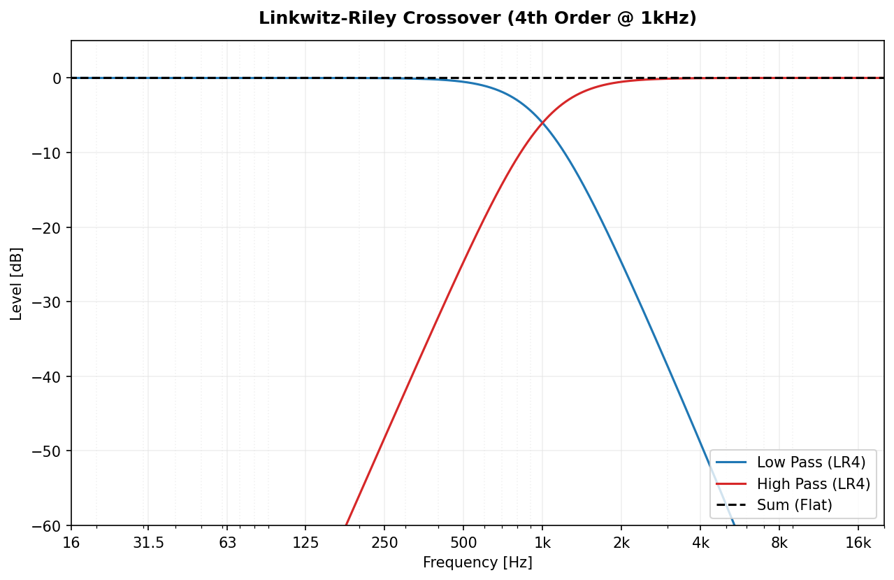
6. Linkwitz-Riley (lr)
Specifically designed for audio crossovers. Linkwitz-Riley filters (typically 4th order) allow splitting a signal into bands that, when summed, result in a perfectly flat magnitude response and zero phase difference between bands at the crossover.
from pyoctaveband import linkwitz_riley
# Split signal into Low and High bands at 1000 Hz
low, high = linkwitz_riley(signal, fs, freq=1000, order=4)
# Reconstruction: low + high == signal (flat response)
📏 Calibration and dBFS
PyOctaveBand can return results in physical Sound Pressure Level (dB SPL) or digital decibels relative to Full Scale (dBFS).
Physical Calibration (Sound Level Meter)
To get accurate SPL measurements from a digital recording, you must first calculate the sensitivity of your measurement chain using a reference tone (e.g., 94 dB @ 1kHz).
from pyoctaveband import octavefilter, calculate_sensitivity

# 1. Record your 94dB calibrator signal
# ref_signal = ... (your recording)

# 2. Calculate sensitivity factor
sensitivity = calculate_sensitivity(ref_signal, target_spl=94.0)

# 3. Apply calibration to your measurements
spl, freq = octavefilter(signal, fs, calibration_factor=sensitivity)
# Now 'spl' values are in real-world dB SPL!
Digital Analysis (dBFS)
...
RMS vs Peak Levels
PyOctaveBand supports two measurement modes to align with professional software like BK:
- RMS (
mode='rms'): Energy-based level (standard). - Peak (
mode='peak'): Absolute maximum value reached in the frame (Peak-holding).
# Measure peak-holding levels for impact analysis
spl_peak, freq = octavefilter(signal, fs, mode='peak')
📊 Signal Decomposition and Stability
By setting sigbands=True, you can retrieve the time-domain components of each band. This is useful for advanced analysis or signal reconstruction.
import numpy as np
from pyoctaveband import octavefilter

# 1. Generate a signal (Sum of 250Hz and 1000Hz)
fs = 8000
t = np.linspace(0, 0.5, fs // 2, endpoint=False)
y = np.sin(2 * np.pi * 250 * t) + np.sin(2 * np.pi * 1000 * t)

# 2. Filter into octave bands and get time-domain signals (sigbands=True)
spl, freq, xb = octavefilter(y, fs=fs, fraction=1, sigbands=True)

# 'xb' is a list of arrays, where xb[i] is the signal filtered in band freq[i]
# Each band in 'xb' has the same length as the original input 'y'.
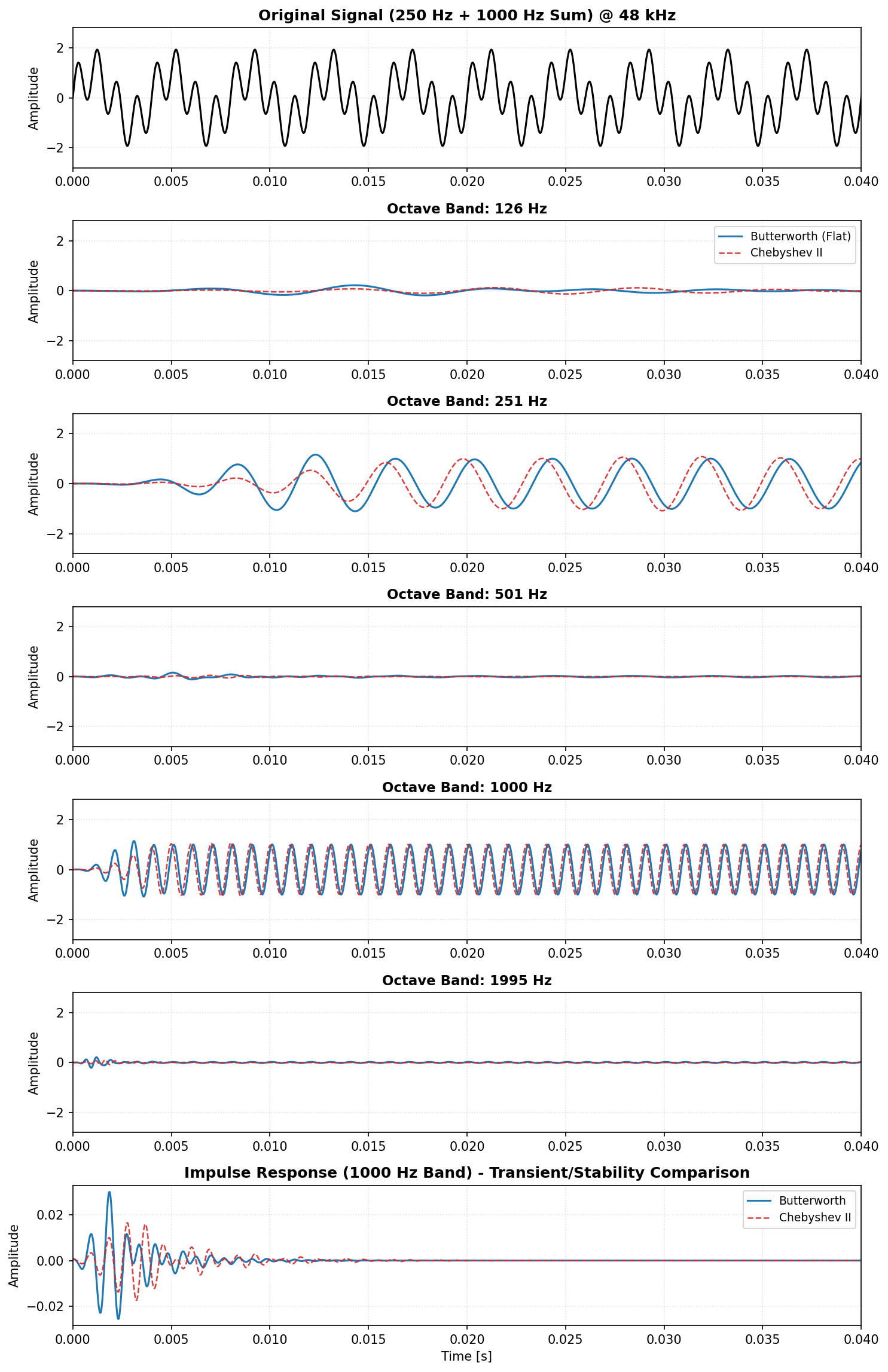
The bottom plot shows the Impulse Response of a band, demonstrating the stability and decay characteristics of the filter.
📖 Theoretical Background
Octave Band Frequencies (ANSI S1.11 / IEC 61260)
The mid-band frequencies ($f_m$) and edges ($f_1, f_2$) use a base-10 ratio $G = 10^{0.3}$:
- Mid-band: $f_m = 1000 \cdot G^{x/b}$ (for odd $b$)
- Band edges: $f_1 = f_m \cdot G^{-1/2b}$, $f_2 = f_m \cdot G^{1/2b}$
Magnitude Responses $|H(j\omega)|$
- Butterworth: $|H(j\omega)| = \frac{1}{\sqrt{1 + (\omega/\omega_c)^{2n}}}$ (Maximally flat)
- Chebyshev I: $|H(j\omega)| = \frac{1}{\sqrt{1 + \epsilon^2 T_n^2(\omega/\omega_c)}}$ ($T_n$ is Chebyshev polynomial)
- Elliptic: $|H(j\omega)| = \frac{1}{\sqrt{1 + \epsilon^2 R_n^2(\omega/\omega_c, L)}}$ ($R_n$ is Jacobian elliptic function)
Weighting Curves (IEC 61672-1)
The A-weighting transfer function: $$R_A(f) = \frac{12194^2 \cdot f^4}{(f^2 + 20.6^2)\sqrt{(f^2 + 107.7^2)(f^2 + 737.9^2)}(f^2 + 12194^2)}$$ $$A(f) = 20 \log_{10}(R_A(f)) + 2.00$$
Time Integration
Implemented as a first-order IIR exponential integrator: $$y[n] = \alpha \cdot x^2[n] + (1 - \alpha) \cdot y[n-1]$$ $$\alpha = 1 - e^{-1 / (f_s \cdot \tau)}$$
🧪 Development and Verification
We maintain 100% stability and compliance through a rigorous test suite.
Test Categories
- Isolation Tests: Verifies that a pure 1kHz tone is attenuated by >20dB in the 250Hz and 4kHz bands.
- Weighting Response: Checks gains at 100Hz (-19.1dB for A) and 1kHz (0dB).
- Stability (IR Tail): Analyzes the Impulse Response of every filter. Energy in the last 100ms must be $< 10^{-6}$ to pass.
- Crossover Flatness: Verifies that the sum of Linkwitz-Riley bands has $< 0.1$ dB deviation.
Commands
# Run full suite
pytest tests/

# Generate technical report
python scripts/benchmark_filters.py
Author
Jose M. Requena Plens, 2020 - 2026.
Release history Release notifications | RSS feed


Download files
Download the file for your platform. If you're not sure which to choose, learn more about installing packages.
Source Distribution
Built Distribution
Filter files by name, interpreter, ABI, and platform.
If you're not sure about the file name format, learn more about wheel file names.
Copy a direct link to the current filters
File details
Details for the file pyoctaveband-1.0.3.tar.gz.
File metadata
- Download URL: pyoctaveband-1.0.3.tar.gz
- Upload date:
- Size: 38.6 kB
- Tags: Source
- Uploaded using Trusted Publishing? No
- Uploaded via: twine/6.2.0 CPython/3.13.11
File hashes
| Algorithm | Hash digest | |
|---|---|---|
| SHA256 |
8f035e8b5759a7374483e24a38463a912fcb63cf47a352abb5c242513dcc4081
|
|
| MD5 |
e7c756282dc5bc352c747e7eda2ffa8a
|
|
| BLAKE2b-256 |
64332943768727aa20802a79cd73d9bc442dc64b92982bd0ff2a7caacc660ef3
|
File details
Details for the file pyoctaveband-1.0.3-py3-none-any.whl.
File metadata
- Download URL: pyoctaveband-1.0.3-py3-none-any.whl
- Upload date:
- Size: 29.3 kB
- Tags: Python 3
- Uploaded using Trusted Publishing? No
- Uploaded via: twine/6.2.0 CPython/3.13.11
File hashes
| Algorithm | Hash digest | |
|---|---|---|
| SHA256 |
6df634cb84bc97b74ab7627ffc7eb2737737fe185370ad8a46c5db2f27894482
|
|
| MD5 |
b6a1b40c8c831c3369634788435b5ce1
|
|
| BLAKE2b-256 |
fdc92df2d0b6201f4421361624e3e009b13e9cd1a085dfa651a3864e43e9ed56
|


