An Open-Source Extensible Package for Simulating Various Statistical Distributions through a Multi-Dimensional Variational Quantum Galton Board!

Project description
QGBx

"Nature isn't classical, dammit, and if you want to make a simulation of nature, you'd better make it quantum mechanical"
QGBx is an open-source, extensible package designed as a submission for the Project 1: "Quantum Walks and Monte Carlo" hosted by the Wiser-Womanium Quantum Summer Program. This package serves as a sandbox for generating several statistical distributions using different Variational Multi-Dimensional Quantum Galton Board architectures, mainly derived from the Universal Statistical Distribution paper by Mark Carney & Ben Varcoe., along with the authors’ efforts to optimize its structure and results for various uses under different noiseless and noisy quantum simulations and even an end-point to run the generated circuits on a real QPU.
Installation
You can install QGBx using
pip install --upgrade QGBx
Usage
QGBx was designed to be extensible in the future, where other Distributions, Devices, Visualization, and Analysis methods can be supported through the same architecture for educational purposes of studying the behavior of the Galton board under both classical and quantum physics, where it was proven that it may help to achieve universal statistical simulators and probability distributions' encoders.
The diagram below shows the relationship between the different objects and the steps of creating, simulating, and retrieving results using QGBx:
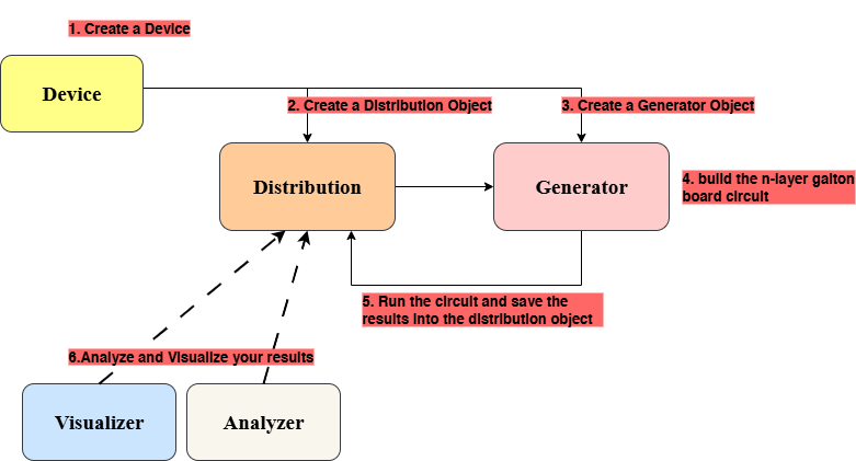
1. Creating a Device:
QGBx supports two kinds of Device: Simulators and Real Devices.
-
Simulators
- Noiseless all-to-all simulators:
PennylanDefaultQubitandQiskitAerSimulator. - Noisy simulator:
QiskitFakeTorino— simulates the noise effects of the Heron IBM Torino device.
- Noiseless all-to-all simulators:
-
Real Devices
IBM_Torino: Runs your generated circuit on the real QPU.Requires a personal IBM token and a CRN code for a created instance.
You can create a device object using QGBx as follows:
# Import the desired device class
from QGBx.devices import QiskitAerSimulator, PennylanDefaultQubit, QiskitFakeTorino, IBM_Torino

# Create a PennylanDefaultQubit device (noiseless simulator)
dev = PennylanDefaultQubit(shots=1000)

# Create a QiskitAerSimulator device (noiseless simulator)
dev = QiskitAerSimulator(shots=1000)

# Create a QiskitFakeTorino device (noisy simulator replicating IBM Torino)
dev = QiskitFakeTorino(ai_optimized=False, optimization_level=0, ai_optimization_level=0, shots=1000)

# Create an IBM_Torino device (real QPU) - requires IBM token and CRN code
dev = IBM_Torino(token="YOUR_IBM_TOKEN", instance_CRN="YOUR_CRN_CODE", optimization_level=1, shots=1000)
Note:
shots: The number of circuit executions (measurements).optimization_level: Qiskit's built-in preset pass manager circuit optimization level (0–3). Higher values can reduce circuit depth but may change gate structure.ai_optimized: Boolean (True/False). Enables or disables the generate_ai_pass_manager.ai_optimization_level: QGBx's AI-based optimization level (0–3). Controls how much the ai_pass manager try to optimize circuit depth and transpilation.
2. Creating a Distribution
QGBx supports three built-in distributions:
Gaussian— Which is essentially a binomial distribution that converges toward a Gaussian distribution under the Laplace–de Moivre theorem when the number of layers of the Galton board becomes large.
Note:
-Distributionobject should take a device as the first parameter :)
from QGBx.distributions import Gaussian

# p is a parameter of the binomial distribution that controls its bias (0.5 is centered)
dist = Gaussian(dev, p=0.4)
Exponential— A distribution where the probabilities follow an exponential decay pattern, defined by a rate parameter (λ).
from QGBx.distributions import Exponential

# rate is λ (lambda) of the exponential function
dist = Exponential(dev, rate=0.5)
Hadamard_QW— A quantum walk distribution generated by Hadamard operations, with different types that define the result of the walk (related to the input state — see the literature for more).
from QGBx.distributions import HadamardQW

# type defines the result of the Hadamard walk (related to the input state)
# type options: ["Symmetric", "Asymmetric_Right", "Asymmetric_Left"]
dist = HadamardQW(dev, type="Symmetric")
The distribution object will then be filled with the results of the simulation and its ideal (theoretical) counterpart in the next step.
The package also gives the user the ability to create a custom Galton board by manipulating the probabilities of pegs in two ways:
- Per peg — each individual peg of the Galton board gets its own probability (of going left or right) using
PegControlled. - Per layer — all pegs of the same layer get the same probability using
LayerControlled(not yet tested).
The user can give specific probabilities for each peg (or layer) or can set a target probability they want, and the package will try to numerically (variationally) tune the pegs (or layers) for that specific target (if possible) using the least squares method.
The user can also directly define the angles of the RX gates. See the structure of the circuits to better understand.
For this distribution the target probabilities "target=" (and effectively the angles "angles=") should be a list encoded as shown in the picture below:
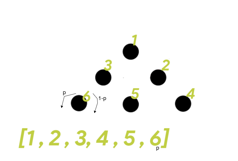
The code for it is like the following:
from QGBx.distributions import PegControlled

# probs (and angles) should be a list encoded as shown in the picture above
dist = PegControlled(device, angles=None, probs=None, optimizer="least_squares", target=None)
There are also the GaussianOp and ExponentialOp, which follow the same logic of the Galton board but use another circuit designed by the authors for the purpose of the Project. This alternative design overcomes many shortcomings in circuit depth and efficiency compared to the main one proposed in the Universal Statistical Simulator method.
They can be instantiated as follows:
from QGBx.distributions import ExponentialOp, GaussianOp

dist = ExponentialOp(dev, rate=0.5) # rate is λ (lambda) of the exponential function

dist = GaussianOp(dev, p=0.4) # p is a parameter of the binomial distribution that controls its bias (0.5 is centered)
3. Creating a Generator
In this package, the Generator is the orchestrator that creates the circuit for a specific Quantum Galton Board architecture to achieve a given Distribution using a chosen Device.
It can be instantiated as follows:
import QGBx

gen = QGBx.Generator(dev, dist)
After that, it provides the user with the following methods:
galton_board(n_layers)
Build the Galton Board circuit.
Parameters:
n_layers(int) – Number of layers in the Galton Board.
Returns:
- Quantum circuit object – The constructed Galton Board circuit and it will automatically assign the circuit to the device, and will be ready for the running phase
run()
Execute the Galton Board circuit on the configured device.
Returns:
dict– One-hot probability distribution from execution and will assign the measured probabilities to the Distribution object, and calculate the ideal probabilities and assign them to the same.
job_results(jobID)
Retrieve results for a given IBM job ID after using the job on the real device is completed (it may take time if the QPU is busy).
Parameters:
jobID(str): IBM Quantum job ID.
Returns:
dict– One-hot probability distribution.
export_circuit_as_png(fold=-1, filename="circuit.png", style="black_white")
Export the circuit diagram as a PNG image.
Parameters:
fold(int): Folding parameter for circuit visualization. set to 25 if you want the circuit to be splitted (only with qiskit circuits)filename(str): Output filename (and directory)style(str): Diagram style. Only the supported
draw_circuit(fold=-1)
Draw the circuit using the device's visualization method.
Parameters:
fold(int): Folding parameter for circuit visualization. set to 25 if you want the circuit to be splitted (only with qiskit circuits)
export_qasm(version="2", filename="exported_circuit.txt")
Export the circuit as a QASM file (only with qiskit circuits)
Parameters:
version(str): QASM version. "2" or "3"filename(str): Output filename (and directory)
4. Generating the n_layers galton board:
This step can be achieved through the genertaor .galton_board(n_layers) method as follow:
n_layers = 6
gen.galton_board(n_layers) #bigger n_layers (more than 6 in some machines) will become computaionally hard if not used the Optimized circuit
- it will automatically assign the circuit to the device, and will be ready for the running
6. Running the circuit:
This step can be achieved through the genertaor .run() method as follow:
gen.run()
- This will assign the measured probabilities to the Distribution object, and calculate the ideal probabilities and assign them to the same.
5. Analyze and Visualize the Results
After retrieving the measured and the ideal theoretical distributions, we can visualize the results through plotting, and analyze the circuit's performance by comparing the measured and the ideal distributions using different metrics.
Visualizing:
QGBx includes a Visualizer object that takes a Distribution object when instantiated, and gives the user the ability to:
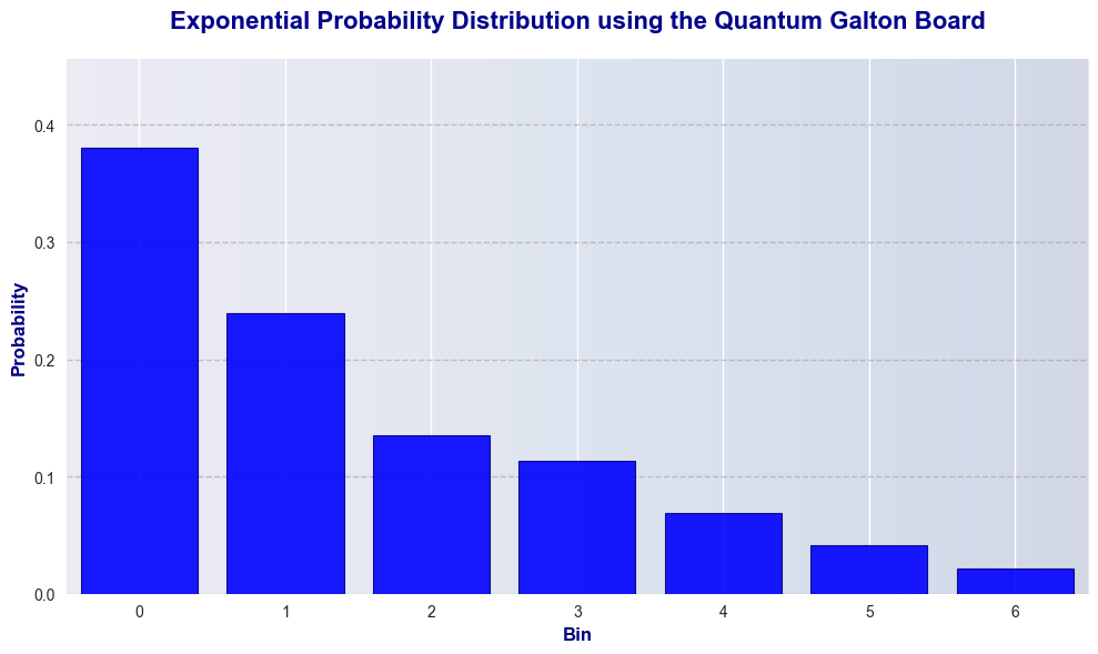
plot(interval_length=None, ideal=False)
Plot the probability distribution (measured or ideal if "ideal" = True)
Parameters:
- interval_length (int, optional): Number of bins to display.
- ideal (bool): Whether to plot the ideal distribution instead of measured.
This can be achieved through:
QGBx.Visualiser(dist).plot()
this will result in the following:
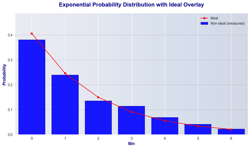
plot_with_ideal(interval_length=None)
Plot the measured probability distribution with the ideal distribution overlaid as points connected with lignes
Parameters:
- interval_length (int, optional): Number of bins to display.
- ideal (bool): Whether to plot the ideal distribution instead of measured.
This can be achieved through:
QGBx.Visualiser(dist).plot_with_ideal()
this will result in the following:
Analyzing:
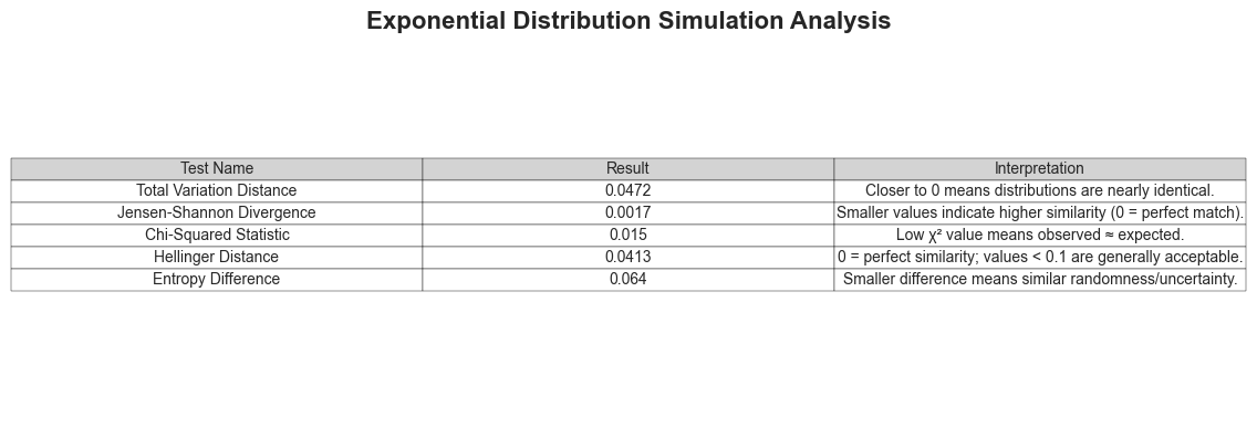
QGBx includes the Analyzer object that takes a Distribution object when instantiated that give the ability to benchmark the measured probability distribution against the ideal theoretical one to assess the accuracy of the circuit and the method through various metrics, and can print a summary of the results.
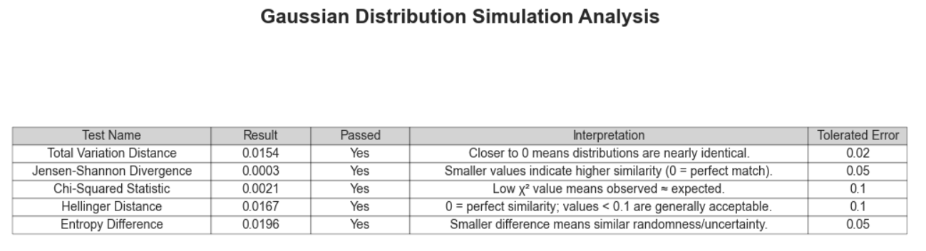
This object also gives the user the ability to define a tolerance for each test in order to generate a report indicating whether the circuit achieved satisfactory results.
The Analyzer have the following methods:
| Method | Description |
|---|---|
total_variation_distance() |
Calculate the Total Variation Distance (TVD) between the ideal (theoritical) and measured distributions. TVD measures the largest possible probability difference between two distributions. Values closer to 0 indicate high similarity. |
jensen_shannon_divergence() |
Calculate the Jensen–Shannon Divergence (JSD) between the ideal (theoritical) and measured distributions. JSD is symmetric and bounded between 0 and 1. A value close to 0 means the distributions are identical. |
chi_squared_test() |
Calculate the Chi-Squared statistic. Smaller values indicate that the measured results are close to the ideal distribution. |
hellinger_distance() |
Calculate the Hellinger Distance between the ideal and quantum distributions. Values range between 0 (identical) and 1 (maximally different). Values < 0.1 are generally acceptable. |
entropy_difference() |
Calculate the absolute difference in Shannon entropy between the ideal and measured distributions. it measures randomness and uncertaintywhere smaller differences mean the distributions have similar uncertainty levels. |
analyze(thresholds=None, show_passed=True) |
Run all analysis metrics and display results in a matplotlib table. Updates pass/fail status using thresholds and displays a formatted table of results. |
get_analyze_results() |
Return the results of the last analysis as a dictionary. If analyze() hasn't been run, it is executed automatically without displaying the table. |
This object can be used in the defined pipeline as follow:
Analyzer = QGBx.Analyzer(dist)
Analyzer.analyze(show_passed=False)
This will results in the following output summary:
The user can also define thresholds and compare the results to the:
Analyzer = QGBx.Analyzer(dist)
Analyzer.analyze(thresholds = [0.02,0.05,0.1,0.1,0.05], show_passed=True)
This will results in the following output summary:
Release history Release notifications | RSS feed


Download files
Download the file for your platform. If you're not sure which to choose, learn more about installing packages.
Source Distribution
Built Distribution
Filter files by name, interpreter, ABI, and platform.
If you're not sure about the file name format, learn more about wheel file names.
Copy a direct link to the current filters
File details
Details for the file qgbx-0.1.1.tar.gz.
File metadata
- Download URL: qgbx-0.1.1.tar.gz
- Upload date:
- Size: 36.9 kB
- Tags: Source
- Uploaded using Trusted Publishing? No
- Uploaded via: twine/6.1.0 CPython/3.12.9
File hashes
| Algorithm | Hash digest | |
|---|---|---|
| SHA256 |
362a263f534b87c2ee3bf0d9f73be370c09d759f846c99af1790c1c1941812b9
|
|
| MD5 |
f0971138f28792e61c4cf77e20f7e56f
|
|
| BLAKE2b-256 |
60d468d6a7f1d28d315bbc00d67982ab5fa3b85fcb60af8b221809ec52af5daa
|
File details
Details for the file qgbx-0.1.1-py3-none-any.whl.
File metadata
- Download URL: qgbx-0.1.1-py3-none-any.whl
- Upload date:
- Size: 42.2 kB
- Tags: Python 3
- Uploaded using Trusted Publishing? No
- Uploaded via: twine/6.1.0 CPython/3.12.9
File hashes
| Algorithm | Hash digest | |
|---|---|---|
| SHA256 |
e55c3eacd3ad92d15769a68fd67683b2bfcaae60cb88afe2ff73aadef106e1eb
|
|
| MD5 |
43a10a48fa69b15a4c15ac4d2e246eee
|
|
| BLAKE2b-256 |
0e3f150c78d2a61913e3f74caf6af7fde58b89b3272ac60e1a8b33374e1f1493
|


