A small package including a one-dimensional well-balanced Shallow Water Equations solver.

Project description
Shallow Water Equations Solver
This package provides a well-balanced solver for the one-dimensional Saint-Venant equations, based on the principles outlined in this paper.
Usage
To utilize this package, you can call the `SWE_Plot`` function with the following parameters:
h, u = SWE_Plot(B, h0, u0, Nx, tEnd, times, g=1, method='C')
Parameters:
- B (callable): Bottom topography function. This function defines the topographic profile and should take spatial coordinates as input and return the bottom elevation at those coordinates. In case of method 'A', should be an array of two callables, representing B and its derivative.
- h0 (array): Initial water height profile. This should be an array of length Nx, representing the initial water height at different spatial locations.
- u0 (array): Initial water velocity profile. Similar to h0, this should be an array of length Nx, representing the initial water velocity at different spatial locations.
- Nx (int): Number of spatial grid points.
- tEnd (float): End time of the simulation. The simulation starts at time t=0.
- times (list): List of time points at which you want to visualize the results.
- g (float, optional): Gravitational constant. Default is 1.
- method (str, optional): Method selection ('A', 'B' or 'C'). Default is 'C'.
Returns:
- h (array): Array containing the water height profile at the final time point.
- u (array): Array containing the water velocity profile at the final time point.
Example:
B = lambda x: 1
f = lambda T: 1 + sqrt(3) / (1 - erf(-0.5 / 0.1)) * (erf((T - 0.5) / 0.1) - erf (-0.5 / 0.1))
h0 = [f(_/ (Nx-1)) for _ in range(Nx)]
u0 = [2.0 / h0[_] for _ in range(Nx)]
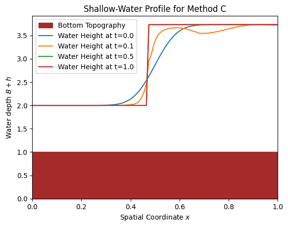
_ = SWE_Plot(B, h0, u0, Nx=100, tEnd=1.0, times=[0.0, 0.1, 0.5, 1.0])
In this example, we're using a spatial grid with 100 points, running the simulation up to t=1 seconds, with gravitational constant g=1 (default value), and visualizing the results at times 0.0, 0.1, 0.5 and 1.0 seconds using method 'C'.
This produces the result in the following figure.
Release history Release notifications | RSS feed


Download files
Download the file for your platform. If you're not sure which to choose, learn more about installing packages.
Source Distribution
Built Distribution
Filter files by name, interpreter, ABI, and platform.
If you're not sure about the file name format, learn more about wheel file names.
Copy a direct link to the current filters
File details
Details for the file SWE_Solver-0.0.2.tar.gz.
File metadata
- Download URL: SWE_Solver-0.0.2.tar.gz
- Upload date:
- Size: 7.2 kB
- Tags: Source
- Uploaded using Trusted Publishing? No
- Uploaded via: twine/4.0.2 CPython/3.11.5
File hashes
| Algorithm | Hash digest | |
|---|---|---|
| SHA256 |
fc9d2184213d6f3367a7683e33365ed8ffc898a32fa3912cf98f524a7f115417
|
|
| MD5 |
785b86761673a6e2db7d5e613bb33934
|
|
| BLAKE2b-256 |
5fd341ec23b2c27d0597d2f2ae3d1bb30802307e6877818c0df855babd1ad180
|
File details
Details for the file SWE_Solver-0.0.2-py3-none-any.whl.
File metadata
- Download URL: SWE_Solver-0.0.2-py3-none-any.whl
- Upload date:
- Size: 7.4 kB
- Tags: Python 3
- Uploaded using Trusted Publishing? No
- Uploaded via: twine/4.0.2 CPython/3.11.5
File hashes
| Algorithm | Hash digest | |
|---|---|---|
| SHA256 |
f68547b5205090d29570d32c7cdb64e81f30a6d1552d7f636a8077cd63f7f97b
|
|
| MD5 |
3a03d8b8841929f33a35ede5618e98c2
|
|
| BLAKE2b-256 |
10e74331874935cfafb814bc74079bcd2e280ba441d3bffd42d73266da135b18
|


