Thermodynamic properties of the phases of H2O and NaCl (aq)


Project description
SeaFreeze
V1.1.3
The SeaFreeze package allows to compute the thermodynamic and elastic properties of water and ice polymorphs (Ih, II, III, V, VI and ice VII/ice X) in the 0-100 GPa and 220-10000 K range, with the study of icy worlds and their ocean in mind. It is based on the evaluation of Gibbs Local Basis Functions parametrization (https://github.com/jmichaelb/LocalBasisFunction) for each phase. The formalism is described in more details in Brown (2018), Journaux et al. (2019), and in the liquid water Gibbs parametrization by Bollengier, Brown, and Shaw (2019).
Installation
This package will install SeaFreeze, LBFTD, and MLBspline and their dependencies.
Requires Python ≥ 3.11.
Run the following command to install:
pip install SeaFreeze
To upgrade to the latest version:
pip install --upgrade SeaFreeze
getProp
Calculates thermodynamic and elastic properties of a phase of water or solution.
Usage
The main function of SeaFreeze is getProp, which has the following parameters:
PT: the pressure (MPa) and temperature (K) conditions at which the thermodynamic quantities should be calculated -- note that these are required units, as conversions are built into several calculations This parameter can have one of the following formats:- a 1-dimensional numpy array of tuples with one or more scattered (P,T) tuples
- a numpy array with 2 nested numpy arrays, the first with pressures and the second with temperatures -- each inner array must be sorted from low to high values a grid will be constructed from the P and T arrays such that each row of the output will correspond to a pressure and each column to a temperature
phase: indicates the phase of H₂O. Supported phases are'Ih'— ice Ih; Feistel & Wagner 2006'II'— ice II; Journaux et al. 2020'III'— ice III; Journaux et al. 2020'V'— ice V; Journaux et al. 2020'VI'— ice VI; Journaux et al. 2020'VII_X_French'— ice VII / ice X; French & Redmer 2015'water1'— liquid water ≤ 500 K, ≤ 2300 MPa; Bollengier et al. 2019 (recommended for 200–355 K)'water2'— liquid water up to 100 GPa; Brown 2018'water_IAPWS95'— IAPWS-95; Wagner & Pruss 2002'NaClaq'— stitched LP+HP NaCl(aq), P=[0, 10001] MPa, T=[229, 2001] K (recommended for NaCl)'NaClaq_LP'— 2026 low-P NaCl(aq) spline only, P=[0, 1001] MPa'NaClaq_HP'— 2026 high-P NaCl(aq) spline only, P=[500, 10001] MPa'NaClaq_5GPa_2024'— legacy Brown 2024 NaCl(aq) spline, P=[0, 5000] MPa
The output of getProp is a SimpleNamespace object whose attributes match those of the Matlab SF_getprop function exactly.
Pass verbose=True to print lbftd diagnostic warnings (e.g. extrapolation outside the spline domain); silent by default.
Deprecation note:
seafreeze.seafreeze()(the old function name) still works but emits aDeprecationWarningand will be removed after 2026-06-21. UsegetPropinstead.
All phases (pure water/ice and NaClaq):
| Quantity | Symbol | Unit |
|---|---|---|
| Gibbs Energy | G |
J/kg |
| Entropy | S |
J/K/kg |
| Internal Energy | U |
J/kg |
| Enthalpy | H |
J/kg |
| Helmholtz free energy | A |
J/kg |
| Density | rho |
kg/m³ |
| Isobaric heat capacity | Cp |
J/kg/K |
| Isochoric heat capacity | Cv |
J/kg/K |
| Isothermal bulk modulus | Kt |
MPa |
| Pressure derivative of Kt | Kp |
− |
| Isentropic bulk modulus | Ks |
MPa |
| Thermal expansivity | alpha |
1/K |
| Bulk sound speed | vel |
m/s |
| Adiabatic temperature gradient | Js |
K/MPa |
| Grüneisen parameter | gamma_Gruneisen |
− |
| Pressure echo | P |
MPa |
| Temperature echo | T |
K |
Solid ice phases additionally (Ih, II, III, V, VI, VII_X_French):
| Quantity | Symbol | Unit |
|---|---|---|
| Shear modulus | shear |
MPa |
| P-wave velocity | Vp |
m/s |
| S-wave velocity | Vs |
m/s |
NaClaq additionally (NaClaq, NaClaq_LP, NaClaq_HP, NaClaq_5GPa_2024):
| Quantity | Symbol | Unit |
|---|---|---|
| Solute chemical potential | mus |
J/mol |
| Solvent (water) chemical potential | muw |
J/mol |
| Partial molar volume of solute | Va |
cm³/mol |
| Apparent molar heat capacity | Cpa |
J/mol/K |
| Partial molar volume | Vm |
cm³/mol |
| Partial molar volume of water | Vw |
cm³/mol |
| Partial molar heat capacity | Cpm |
J/mol/K |
| Osmotic coefficient | phi |
− |
| Excess volume | Vex |
cm³/mol |
| Water activity | aw |
− |
| Molality echo | m |
mol/kg |
| Solute mole fraction | xs |
− |
| Solvent mole fraction | xw |
− |
| Mass fraction factor | f |
kg-soln/kg-H₂O |
NaN values are returned for conditions outside the parametrization boundaries.
Example
import numpy as np
from seafreeze import seafreeze as sf

# list supported phases
sf.phases.keys()

# evaluate thermodynamics for ice VI at 900 MPa and 255 K
PT = np.empty((1,), dtype='object')
PT[0] = (900, 255)
out = sf.getProp(PT, 'VI')
# view a couple of the calculated thermodynamic quantities at this P and T
out.rho     # density
out.Vp      # compressional wave velocity

# evaluate thermodynamics for water at three separate PT conditions
PT = np.empty((3,), dtype='object')
PT[0] = (441.0858, 313.95)
PT[1] = (478.7415, 313.96)
PT[2] = (444.8285, 313.78)
out = sf.getProp(PT, 'water1')
# values for output fields correspond positionally to (P,T) tuples
out.H       # enthalpy

# evaluate ice V thermodynamics at pressures 400-500 MPa and temperatures 240-250 K
P = np.arange(400, 501, 2)
T = np.arange(240, 250.1, 0.5)
PT = np.array([P, T], dtype='object')
out = sf.getProp(PT, 'V')
# rows in output correspond to pressures; columns to temperatures
out.A       # Helmholtz energy
out.shear   # shear modulus
seafreeze.whichphase: determining the stable phase of water
Usage
SeaFreeze includes a function to determine which of the supported phases is stable under the given pressure and temperature conditions.
whichphase(PTm, solute='water1', path=defpath)
PTm— same format asgetProp(PTfor pure water,PTmfor NaCl solutions)solute— optional; set to'NaCl'to use NaClaq as the liquid phase, enabling freezing-point-depression phase maps;PTmthen requires a molality axis[P, T, m]
The output is a NumPy array of integers: 0 = liquid, 1 = ice Ih, 2 = II, 3 = III, 5 = V, 6 = VI; numpy.nan outside all parametrizations.
- Scattered (P,T): each value corresponds to the same index in the input
- Grid: each row corresponds to a pressure and each column to a temperature
phasenum2phase(phaseInt) converts an integer phase number back to a material string.
Example
import numpy as np
from seafreeze import seafreeze as sf

# determine the phase of water at 900 MPa and 255 K
PT = np.empty((1,), dtype=object)
PT[0] = (900, 255)
out = sf.whichphase(PT)
# map to a phase using phasenum2phase
sf.phasenum2phase(out[0])

# determine phase for three separate (P,T) conditions
PT = np.empty((3,), dtype=object)
PT[0] = (100, 200)
PT[1] = (400, 250)
PT[2] = (1000, 300)
out = sf.whichphase(PT)
# show phase for each (P,T)
[(pt, sf.phasenum2phase(pn)) for (pt, pn) in zip(PT, out)]

# find the likely phases at pressures 0-5 MPa and temperatures 240-300 K
P = np.arange(0, 5, 0.1)
T = np.arange(240, 300)
PT = np.array([P, T], dtype=object)
out = sf.whichphase(PT)

# phase map for a 2 mol/kg NaCl solution (freezing-point depression)
PTm = np.array([np.arange(0, 500, 10), np.arange(240, 300, 0.6),
                np.full(50, 2.0)], dtype=object)
out = sf.whichphase(PTm, solute='NaCl')
Phase boundaries: seafreeze.phaselines
SeaFreeze 1.1.0 adds a dedicated module for computing and plotting phase boundary curves — the equilibrium (P, T) loci between any two supported phases. It is the Python equivalent of the Matlab SF_PhaseLines / SF_WPD stack.
Public API
| Function | Returns | Description |
|---|---|---|
phase_range(material) |
PhaseRange(P, T, m) |
Knot-domain bounds of the Gibbs spline for one material |
phase_lines(matA, matB, …) |
PhaseLineResult (or list) |
Equilibrium (P, T) curve between two phases |
wpd(…) |
matplotlib.figure.Figure |
Full water phase diagram plot |
phase_lines parameters
| Parameter | Default | Description |
|---|---|---|
matA, matB |
— | Phase names (same as getProp; order does not matter) |
m |
None |
Molality (mol/kg) — required when one phase is 'NaClaq'; accepts a scalar or list; m=0 gives the pure-water limit via the NaClaq EoS |
T |
auto | 1-D array of temperatures (K) to use as the evaluation grid |
segment |
'all' |
'all', 'stable', or 'meta' — which part of the curve to return |
The PhaseLineResult object has attributes matA, matB, P (MPa), T (K), stable (bool mask), segment, and m.
wpd parameters
| Parameter | Default | Description |
|---|---|---|
ax |
None (new figure) |
Matplotlib Axes to plot onto; creates a new figure if omitted |
solute |
'none' |
'NaCl' to overlay NaClaq melting curves |
m |
None |
Molality list for the NaCl overlay |
show_meta |
True |
Show metastable extensions as dashed gray lines |
phase_labels |
False |
Annotate phase fields (Ih, II, III, V, VI, Liquid) |
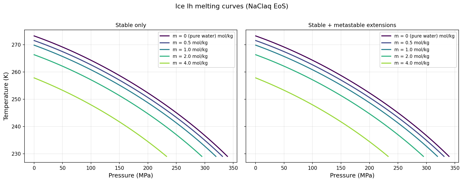
Example — Ice Ih melting curves with NaCl
m=0 uses the NaClaq EoS at the pure-water limit. Higher concentration depresses the melting temperature across the entire pressure range.
import matplotlib.pyplot as plt
import matplotlib.cm as cm
import numpy as np
from seafreeze.phaselines import phase_lines

m_vals   = [0.0, 0.5, 1.0, 2.0, 4.0]
m_labels = ['0 (pure water)', '0.5', '1.0', '2.0', '4.0']
colors   = cm.viridis(np.linspace(0.0, 0.85, len(m_vals)))

fig, ax = plt.subplots(figsize=(7, 5))
for m, lbl, c in zip(m_vals, m_labels, colors):
    r = phase_lines('Ih', 'NaClaq', m=m, segment='stable')
    ax.plot(r.P, r.T, '-', color=c, lw=2, label=f'm = {lbl} mol/kg')
ax.set_xlabel('Pressure (MPa)')
ax.set_ylabel('Temperature (K)')
ax.set_title('Ice Ih melting curves (NaClaq EoS)')
ax.legend(fontsize=9)
ax.grid(True, alpha=0.3)
plt.tight_layout()
plt.show()
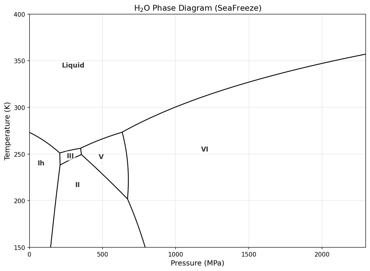
Example — Full pure-water phase diagram
Use show_meta=False to hide metastable extensions and phase_labels=True to annotate each stability field.
from seafreeze.phaselines import wpd

with warnings.catch_warnings():
    warnings.simplefilter('ignore')
    fig = wpd(show_meta=False, phase_labels=True)
plt.show()
wpd also accepts a solute='NaCl' keyword together with a list of molalities to overlay NaCl melting curves on the diagram:
fig = wpd(show_meta=False, phase_labels=True, solute='NaCl', m=[0.5, 2.0, 4.0])
EOS inversion: seafreeze.rho2P
rho2P inverts the SeaFreeze EOS to find pressure P (MPa) such that rho(P, T) == rho_target for any supported material. Uses Newton-Raphson with the isothermal bulk modulus Kt and a bisection fallback for robustness; returns NaN where no solution exists within the spline domain.
Signature
from seafreeze import rho2P

P = rho2P(rho_target, T, phase)
P = rho2P(rho_target, T, phase, m=1.0)          # NaClaq: molality in mol/kg
P = rho2P(rho_target, T, phase, P0=500.0)        # optional initial guess (MPa)
P = rho2P(rho_target, T, phase, tol=1e-4)        # convergence tolerance (default 0.01 MPa)
| Parameter | Description |
|---|---|
rho_target |
Target density in kg/m³ — scalar or array-like |
T |
Temperature in K — scalar broadcasts against rho_target |
phase |
Any material code accepted by getProp |
m |
Molality in mol/kg — required for NaClaq phases |
P0 |
Optional initial pressure guess in MPa |
tol |
Convergence tolerance in MPa (default 0.01) |
Returns a NumPy array of the same shape as rho_target. NaN is returned where no solution was found (density out of range at the given T, or T outside the spline domain).
Example
import numpy as np
from seafreeze import rho2P

# Pure water near ambient conditions
P = rho2P(997.0, 298.0, 'water1')          # ≈ 0.1 MPa

# Ice Ih at 1 bar — works at 0.1 MPa (low-P fix in 1.1.3)
P = rho2P(918.6, 260.0, 'Ih')              # ≈ 0.1 MPa

# Ice VI — three scatter points
P = rho2P([1310., 1350., 1390.], [255., 260., 265.], 'VI')

# NaClaq at 1 mol/kg
P = rho2P(1050.0, 300.0, 'NaClaq', m=1.0)

# Round-trip check: compute rho with getProp, recover P with rho2P
import numpy as np, warnings
from seafreeze import getProp, rho2P
PTm = np.empty(1, dtype=object); PTm[0] = (500., 300.)
rho = getProp(PTm, 'water1').rho.flat[0]
P_rec = rho2P(rho, 300., 'water1')         # should recover ≈ 500 MPa
Important remarks
Water representation
The ice Gibbs parametrizations are optimized to be used with water1 (Bollengier et al. 2019), particularly for phase-equilibrium calculations. Using other water parametrizations will lead to incorrect melting curves. water2 (Brown 2018) and water_IAPWS95 (IAPWS-95) are provided for high-pressure extension (up to 100 GPa) and comparison only. The authors recommend water1 for any application in the 200–355 K range and up to 2300 MPa.
Range of validity
SeaFreeze stability prediction is currently considered valid down to 130K, which correspond to the ice VI - ice XV transition. The ice Ih - II transition is potentially valid down to 73.4 K (ice Ih - ice XI transition). The ice VII and ice X representation extend to 1TPa (1e6 MPa) and 2000K.
References
- Bollengier, Brown and Shaw (2019) J. Chem. Phys. 151, 054501; doi: 10.1063/1.5097179
- Brown (2018) Fluid Phase Equilibria 463, pp. 18-31
- Feistel and Wagner (2006), J. Phys. Chem. Ref. Data 35, pp. 1021-1047
- Journaux et al. (2020) JGR: Planets 125, e2019JE006176
- Wagner and Pruss (2002), J. Phys. Chem. Ref. Data 31, pp. 387-535
- French and Redmer (2015), Physical Review B 91, 014308
Authors
- Baptiste Journaux - University of Washington, Earth and Space Sciences Department, Seattle, USA
- J. Michael Brown - University of Washington, Earth and Space Sciences Department, Seattle, USA
- Penny Espinoza - University of Washington, Earth and Space Sciences Department, Seattle, USA
- Erica Clinton - University of Washington, Earth and Space Sciences Department, Seattle, USA
- Tyler Gordon - University of Washington, Department of Astronomy, Seattle, USA
- Ula Jones - University of Washington, Earth and Space Sciences Department, Seattle, USA
Change log
Changes since 0.9.0
1.1.3: Addedrho2P— EOS pressure-from-density inversion via Newton-Raphson + bisection fallback, supporting all phases including NaClaq. Fixed low-pressure convergence for all ice phases (Ih, II, III, V, VI).1.1.2: Fixed bug in_get_shear_mod_GPawhere temperature was not cast to a numpy array, causingnp.sqrtto fail on 2-D grid inputs for solid phases. All shear-wave properties (shear,Vp,Vs) on grids now compute correctly.1.1.1: Addedmatplotlibto Python dependencies; removednumpy<2upper bound for NumPy 2.x compatibility.1.1.0: addedseafreeze.phaselinesmodule — phase boundary computation (phase_lines,phase_range) and the full water phase diagram plotter (wpd); NaClaq melting curves for Ih, II, III, V, and VI; cross-validated against the Matlab SF_PhaseLines implementation to < 0.01 K.getPropoutput now matches MatlabSF_getpropexactly: addedJs,gamma_Gruneisen,P/Techoes, NaClaq mixing properties (m,xs,xw,f,Vw); removed Python-onlyV,gam,Gexfrom default output; individual per-spline.matfiles replace the monolithic spline archive.1.0: added NaCl aqueous solution EOS and concentration dependent thermodynamic variables.0.9.4: Adjusted python readme syntax and package authorship info0.9.3: add ice VII and ice X from French and Redmer (2015). LocalBasisFunction spline interpretation software integrated into SeaFreeze Python package. Adjusted packaging to work better with pip0.9.2.post2:whichphasereturnsnumpy.nanif PT is outside the regime of all phases0.9.2: add ice II to the representation.0.9.1: addwhichphasefunction
Changes from 0.8
- rename function get_phase_thermodynamics to seafreeze
- reverse order of PT and phase in function signature
- remove a layer of nesting (
seafreeze.seafreezerather thanseafreeze.seafreeze.seafreeze)
License
SeaFreeze is licensed under the GPL-3 License :
Copyright (c) 2019, B. Journaux
This program is free software: you can redistribute it and/or modify it under the terms of the GNU General Public License as published by the Free Software Foundation, version 3.
This program is distributed in the hope that it will be useful, but WITHOUT ANY WARRANTY; without even the implied warranty of MERCHANTABILITY or FITNESS FOR A PARTICULAR PURPOSE. See the GNU General Public License for more details.
You should have received a copy of the GNU General Public License along with this program. If not, see https://www.gnu.org/licenses/.
THERE IS NO WARRANTY FOR THE PROGRAM, TO THE EXTENT PERMITTED BY APPLICABLE LAW. EXCEPT WHEN OTHERWISE STATED IN WRITING THE COPYRIGHT HOLDERS AND/OR OTHER PARTIES PROVIDE THE PROGRAM "AS IS" WITHOUT WARRANTY OF ANY KIND, EITHER EXPRESSED OR IMPLIED, INCLUDING, BUT NOT LIMITED TO, THE IMPLIED WARRANTIES OF MERCHANTABILITY AND FITNESS FOR A PARTICULAR PURPOSE. THE ENTIRE RISK AS TO THE QUALITY AND PERFORMANCE OF THE PROGRAM IS WITH YOU. SHOULD THE PROGRAM PROVE DEFECTIVE, YOU ASSUME THE COST OF ALL NECESSARY SERVICING, REPAIR OR CORRECTION.
Acknowledgments
This work was produced with the financial support provided by the NASA Postdoctoral Program fellowship, by the NASA Solar System Workings Grant 80NSSC17K0775 and by the Icy Worlds node of NASA's Astrobiology Institute (08-NAI5-0021).
Illustration montage uses pictures from NASA Galileo and Cassini spacecrafts (from top to bottom: Enceladus, Europa and Ganymede). Terrestrial sea ice picture use with the authorization of the author Rowan Romeyn.
Project details
Release history Release notifications | RSS feed


Download files
Download the file for your platform. If you're not sure which to choose, learn more about installing packages.
Source Distribution
Built Distribution
Filter files by name, interpreter, ABI, and platform.
If you're not sure about the file name format, learn more about wheel file names.
Copy a direct link to the current filters
File details
Details for the file seafreeze-1.1.3.tar.gz.
File metadata
- Download URL: seafreeze-1.1.3.tar.gz
- Upload date:
- Size: 47.6 MB
- Tags: Source
- Uploaded using Trusted Publishing? No
- Uploaded via: twine/6.2.0 CPython/3.13.9
File hashes
| Algorithm | Hash digest | |
|---|---|---|
| SHA256 |
7a6f061ccc4540cdc2c056401951107e0836bf0a094e532e3348266afa7f7ad7
|
|
| MD5 |
4f6f19878178bf5769353df91b66a932
|
|
| BLAKE2b-256 |
65a6a994e19fb0d0ef594d288bf25d249d0766c2a072e0243ecd7e207fc72d0a
|
File details
Details for the file seafreeze-1.1.3-py3-none-any.whl.
File metadata
- Download URL: seafreeze-1.1.3-py3-none-any.whl
- Upload date:
- Size: 47.6 MB
- Tags: Python 3
- Uploaded using Trusted Publishing? No
- Uploaded via: twine/6.2.0 CPython/3.13.9
File hashes
| Algorithm | Hash digest | |
|---|---|---|
| SHA256 |
59eb1a3e6dc67e40ba17f181c44d85a0f8c958bc6543e2b29a8cf3d060e69fa1
|
|
| MD5 |
b433021e2fa730f9e8f5435cebe4226c
|
|
| BLAKE2b-256 |
c62087f7cb1edeefbe271c13ae6d18623294306c7738bd157175d71db377caa4
|


