A Python package for causal inference using various Synthetic Control Methods

Project description
Synthetic Control Methods
A Python package for causal inference using synthetic controls
This Python package implements a class of approaches to estimating the causal effect of an intervention on panel data or a time-series. For example, how was West Germany's economy affected by the German Reunification in 1990? Answering a question like this can be difficult when a randomized experiment is not available. This package aims to address this difficulty by providing a systematic way to choose comparison units to estimate how the outcome of interest would have evolved after the intervention if the intervention had not occurred.
As with all approaches to causal inference on non-experimental data, valid conclusions require strong assumptions. This method assumes that the outcome of the treated unit can be explained in terms of a set of control units that were themselves not affected by the intervention. Furthermore, the relationship between the treated and control units is assumed to remain stable during the post-intervention period. Including only control units in your dataset that meet these assumptions is critical to the reliability of causal estimates.
Installation
pip install SyntheticControlMethods
Usage
In this simple example, we replicate Abadie, Diamond and Hainmueller (2015) which estimates the economic impact of the 1990 German reunification on West Germany using the synthetic control method. Here is a complete example with explanations (if you have trouble loading the notebook: use this).
#Import packages
import pandas as pd
from SyntheticControlMethods import Synth

#Import data
data = pd.read_csv("examples/german_reunification.csv")
data = data.drop(columns="code", axis=1)

#Fit classic Synthetic Control
sc = Synth(data, "gdp", "country", "year", 1990, "West Germany", pen=0)

#Visualize synthetic control
sc.plot(["original", "pointwise", "cumulative"], treated_label="West Germany",
            synth_label="Synthetic West Germany", treatment_label="German Reunification"))
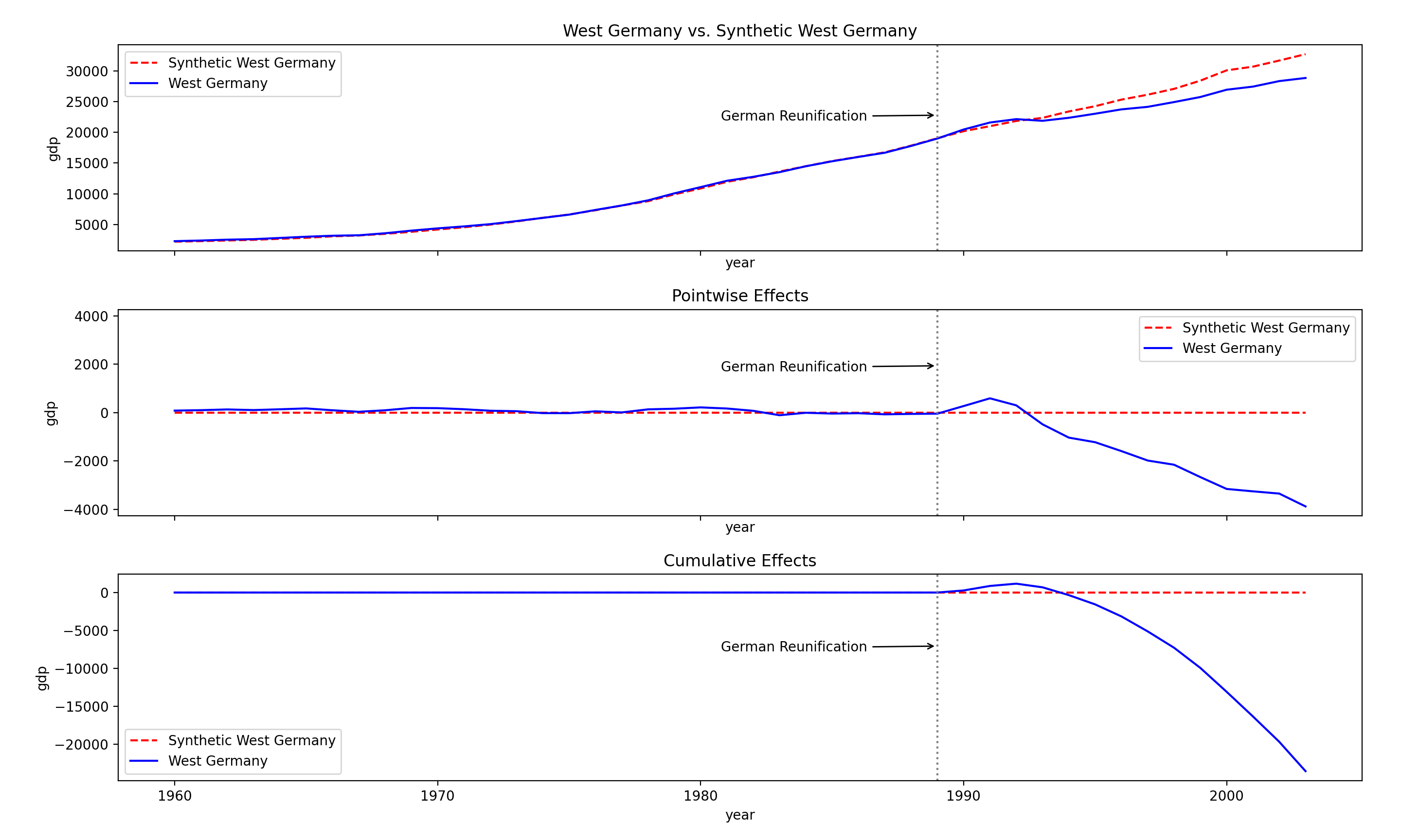
The plot contains three panels. The first panel shows the data and a counterfactual prediction for the post-treatment period. The second panel shows the difference between observed data and counterfactual predictions. This is the pointwise causal effect, as estimated by the model. The third panel adds up the pointwise contributions from the second panel, resulting in a plot of the cumulative effect of the intervention.
More background on the theory that underlies the Synthetic Control
1. The fundamental problem of Causal Inference
In this context, we define the impact or, equivalently, causal effect of some treatment on some outcome for some unit(s), as the difference in potential outcomes. For example, the effect of taking an aspirin on my headache is defined to be the difference in how much my head aches if I take the pill as compared to how much my head would have ached had I not taken it. Of course, it is not possible for me to both take and not take the aspirin. I have to choose one alternative, and will only observe the outcome associated with that alternative. This logic applies to any treatment on any unit: only one of two potential outcomes can ever be observed. This is often referred to as the fundamental problem of causal inference (Rubin, 1974). The objective of models in this package is to estimate this unobserved quantity–what the outcome of the treated unit would have been if it had not received the treatment.
2. The data format
In keeping with the notational conventions introduced in Abadie et al. (2010), consider J+1 units observed in time periods T = {1,2,...,T}. Unit at index 1 is the only treated unit, the remaining J units {2,..,J} are untreated. We define T0 to represent the number of pre-treatment periods and T1 the number post-treatment periods, such that T = T0+ T1. That is, Unit 1 is exposed to the treatment in every post-treatment period, T0+1,...,T1, and unaffected by the treatment in all preceding periods, 1,...,T0. Lastly, we require that a set of covariates–characteristics of the units relevant in explaining the value of the outcome–are observed along with the outcome at each time period. An example dataset might, in terms of structure, look like this:
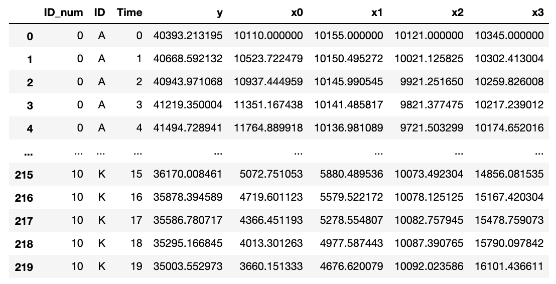
In this example dataset, each row represents an observation. The unit associated with the observation is indicated by the ID column, the time period of the observation by the Time column. Column y represents the outcome of interest and column x0,...,x3 are covariates. There can be an arbitrary, positive number of control units, time periods and covariates.
3. Synthetic Control Model
Conceptually, the objective of the SCM is to create a synthetic copy of the treated unit that never received the treatment by combining control units. More specifically, we want to select a weighted average of the control unit that most closely resembles the pre-treatment characteristics of the treated unit. If we find such a weighted average that behaves the same as the treated unit for a large number of pre-treatment periods, we make the inductive leap that this similarity would have persisted in the absence of treatment.
Any weighted average of the control units is a synthetic control and can be represented by a (J x 1) vector of weights W = (w2,...,wJ+1), with wj ∈ (0,1) and w2 + … + wJ+1 = 1. The objective is this to find the W for which the characteristics of the treated unit are most closely approximated by those of the synthetic control. Let X1 be a (k x 1) vector consisting of the pre-intervention characteristics of the treated unit which we seek to match in the synthetic control. Operationally, each value in X1 is the pre-treatment average of each covariate for the treated unit, thus k is equal to the number of covariates in the dataset. Similarly, let X0 be a (k x J) containing the pre-treatment characteristics for each of the J control units. The difference between the pre-treatment characteristics of the treated unit and a synthetic control can thus be expressed as X1 - X0W. We select W* to minimize this difference.
In practice, however, this approach is flawed because it assigns equal weight to all covariates. This means that the difference is dominated by the scale of the units in which covariates are expressed, rather than the relative importance of the covariates. For example, mismatching a binary covariate can at most contribute one to the difference, whereas getting a covariate which takes values on the order of billions, like GDP, off by 1% may contribute hundreds of thousands to the difference. This is problematic because it is not necessarily true that a difference of one has the same implications on the quality of the approximation of pre-treatment characteristics provided by the synthetic control. To overcome this limitation we introduce a (k x k) diagonal, semidefinite matrix V that signifies the relative importance of each covariate. Lastly, let Z1 be a (1 x T0) matrix containing every observation of the outcome for the treated unit in the pre-treatment period. Similarly, let Z0 be a (k x T0) matrix containing the outcome for each control unit in the pre-treatment period.
The procedure for finding the optimal synthetic control is expressed as follows:
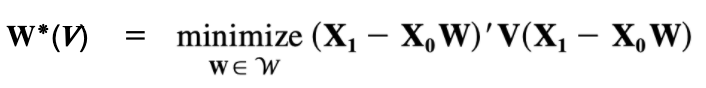
That is, W*(V) is the vector of weights W that minimizes the difference between the pre-treatment characteristics of the treated unit and the synthetic control, given V. That is, W* depends on the choice of V–hence the notation W*(V). We choose V* to be the V that results in W*(V) that minimizes the following expression:
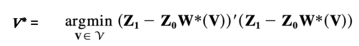
That is the minimum difference between the outcome of the treated unit and the synthetic control in the pre-treatment period.
In code, I solve for W*(V) using a convex optimizer from the cvxpy package, as the optimization problem is convex. I define the loss function total_loss(V) to be the value of Eq.2 with W*(V) derived using the convex optimizer. However, finding V that minimizes total_loss(V) is not a convex problem. Consequently, I use a solver, minimize(method=’L-BFGS-B’) from the scipy.optimize module, that does not require convexity but in return cannot guarantee that the global minimum of the function is found. To decrease the probability that the solution provided is only a local minimum, I initialize the function for several different starting values of V. I randomly generate valid (k x k) V matrices as Diag(K) with K ~ Dirichlet({11,...,1k}).
Input on how to improve the package is welcome, just submit a pull request along with an explanation and I will review it.
Release history Release notifications | RSS feed


Download files
Download the file for your platform. If you're not sure which to choose, learn more about installing packages.
Source Distribution
File details
Details for the file SyntheticControlMethods-1.1.17.tar.gz.
File metadata
- Download URL: SyntheticControlMethods-1.1.17.tar.gz
- Upload date:
- Size: 26.5 kB
- Tags: Source
- Uploaded using Trusted Publishing? No
- Uploaded via: twine/3.4.2 importlib_metadata/3.10.0 pkginfo/1.7.0 requests/2.25.1 requests-toolbelt/0.9.1 tqdm/4.59.0 CPython/3.8.8
File hashes
| Algorithm | Hash digest | |
|---|---|---|
| SHA256 |
941c77427ef1a87d5cf5863047c5d0c77c280a6b3aea04de3302e56fa76fe505
|
|
| MD5 |
edd31a8e869d664dd29ed9e62993089e
|
|
| BLAKE2b-256 |
81b9c87ed26799a76c5627571b3b9ab6344727b01a5ffd7e8dd4062bd6428373
|


