A simulation package for thermodynamic systems

Project description
Chapter 1: Introduction
Overview of the Thermodynamic Model
This Python module, ThermoSim, is designed to simulate and analyze various thermodynamic systems and components. It can model complex systems involving fluids such as water, air, and refrigerants like isobutane. The module supports a range of thermodynamic processes, including pumps, turbines, heat exchangers, and other essential components commonly found in energy systems, refrigeration cycles, and heat transfer applications.
Key Features:
-
State Point Management: The module allows you to define and track state points, representing the thermodynamic properties of fluids (e.g., temperature, pressure, enthalpy) at various points in the system.
-
Component Modeling: It models different components like pumps, turbines, heat exchangers, and expansion valves, each with specific methods for energy calculations and performance evaluation.
This model serves as a powerful tool for engineers and researchers working on thermodynamic cycle design, optimization, and analysis, including heat pumps, refrigeration systems, and other energy conversion systems.
Target Audience
This documentation is intended for:
-
Engineering Students: Those studying thermodynamics, energy systems, and heat transfer. The module provides a practical tool to simulate real-world energy systems and understand thermodynamic concepts.
-
Researchers: Professionals and researchers working in the field of thermodynamics and energy efficiency can use this module for modeling, optimization, and analysis of complex systems.
-
Energy System Designers: Engineers involved in designing and optimizing thermodynamic systems such as power plants, heat exchangers, refrigeration cycles, and renewable energy systems.
Real-World Applications
-
Heat Exchanger Design and Optimization: The module simulates various types of heat exchangers (e.g., double-pipe, evaporator, condenser), helping engineers optimize thermal efficiency and energy usage in industrial applications.
-
Pumps and Turbines: It can model pumps and turbines used in power generation, refrigeration, and HVAC systems, providing insights into performance metrics like work output, efficiency, and energy transfer
-
Energy Efficiency Analysis: By integrating components like expansion valves and PCM (Phase Change Materials), the model supports the design of energy-efficient systems in heating, cooling, and refrigeration sectors.
-
Simulation of Thermodynamic Cycles: The module supports the simulation of thermodynamic cycles, including Rankine and refrigeration cycles, helping in the evaluation of system performance, energy conservation, and operational optimization.
Chapter 2: Installation and Setup
Installation
To install the ThermoSim module, follow the steps below. This module is compatible with Python 3.6+.
Installing via PyPI
You can install the module directly from PyPI using pip:
pip install ThermoSim
Quick Start
Once installed, you can start using the module by importing it into your Python script.
Example Usage
import ThermoSim

# Initialize the thermodynamic model
model = ThermoSim.ThermodynamicModel()

# Define fluid state points
model.add_point('water', StatePointName='1', P=6.09e5, T=158+273.15, Mass_flowrate=555.9)
model.add_point('water', StatePointName='2', P=6.09e5, T=None, Mass_flowrate=555.9)

# Add components (e.g., pump, heat exchanger)
pump = model.Pump(model, 'Pump', In_state='1', Out_state='2', n_isen=0.75, Calculate=True)

print(Model)
Chapter 3: Basic Usage
Creating and Setting Up the Model
This chapter explains how to create the thermodynamic model, define state points, and add components like pumps, turbines, and heat exchangers to simulate thermodynamic systems.
1. The Prop() Function
Before defining state points, let’s understand the Prop() function, as it is used to calculate and create the thermodynamic state for fluids. Prop() is using coolprop for calculating the thermodynamic properties. The Prop() function returns an object (called State) that holds the thermodynamic properties of the fluid at a specific state point.
Here’s how the Prop() function works:
State = model.Prop(fluid, StatePointName, Mass_flowrate=None, **properties)
Arguments for the Prop() function:
-
fluid: The fluid type (e.g., 'water', 'isobutane').
-
StatePointName: A unique identifier for the state point (e.g., '1', '2').
-
Mass_flowrate (optional): The mass flow rate of the fluid at the state point (in kg/s).
-
**properties: These are the thermodynamic properties to define the state point, such as:
- P: Pressure at the state point (in Pascals).
- T: Temperature at the state point (in Kelvin).
- H: Enthalpy at the state point (in J/kg).
- S: Entropy at the state point (in J/kg·K).
- Q: Quality of the fluid (used in two-phase fluids)
- State.D: Density (in kg/m³)
State Object
The Prop() function creates a State object that holds the thermodynamic properties of the fluid. You can access or update the properties of this object directly.
-
State.T: Temperature (in Kelvin)
-
State.P: Pressure (in Pascals)
-
State.H: Enthalpy (in J/kg)
-
State.S: Entropy (in J/kg·K)
-
State.D: Density (in kg/m³)
-
State.Cp: Specific heat at constant pressure (in J/kg·K)
Example Usage of Prop() and Accessing Properties:
# Define a state point for water
State = model.Prop('water', 'Demo', P=6.09e5, T=158 + 273.15)

# Print all properties of the State object
print(State)  # This will display the State object's properties like T, P, H, etc.

# Update the pressure directly
State.P = 7e5  # New pressure in Pascals

# Print updated State object to check changes
print(State)  # The updated properties will be displayed
In this example:
-
State is an object that stores all the thermodynamic properties for the fluid at state point 'Demo’'.
-
We can access the temperature, pressure, enthalpy, entropy, density, and specific heat directly using
State.T,State.P,State.H,State.S,State.D, andState.Cp, respectively. -
We update the pressure of the state point using
State.P = 7e5.
2. Adding State Point to the Model
State points represent the thermodynamic conditions (like pressure, temperature, and mass flow rate) at different points in the system. These points are added using the add_point() method, which internally calls the Prop() function to calculate and store the properties of the fluid.
Adding State Points
When adding a state point, you can define only the known parameters (e.g., pressure, temperature etc.) . The missing properties will be calculated by the model based on the provided values.
# Adding a state point for water with a known pressure only

model.add_point('water', StatePointName='1', P=6.09e5, T= 180+273.15, Mass_flowrate=None)

print(model.Points['1'])
In this example:
-
'water' is the fluid.
-
StatePointName='1' is the unique identifier for the state point.
-
P=6.09e5 sets the pressure.
-
T=180+273.15 sets the themperature.
-
Mass_flowrate=None indicates that the mass flow rate is not specified and can be calculated.
You can also set parameters like pressure (P), Temperature (T), enthalpy (H), entropy (S), quality (Q), and density (D) to None:
# Adding a state point for water with a known pressure only

model.add_point('water', StatePointName='1', P=6.09e5, T= None, Mass_flowrate=None)

print(model.Points['1'])
Here you can see that the state point '1' is added to the model but properties are not calculated as the sufficient numbers of parameters are not given.
State Points in the Model
All the state points you add are stored in model.Point. You can access each state point by its StatePointName and view or update its properties.
# Access a state point by its name (e.g., '1')
State = model.Point['1']

# Print the properties of the state point
print(State)
3. Updating State Points
You can also update the properties of any state point after it has been created. For example, to update the pressure of state point '1', you can do:
# Update the pressure of state point '1'
model.Point['1'].P = 7e5  # Update pressure to 7e5 Pascals

# Print the updated state point to verify the change
print(model.Point['1'])
4. Displaying All State Points
To view all state points and their properties, you can use the model.Point_print() method:
# Print all state points in the model
model.Point_print()
This will display all the state points and their corresponding properties (e.g., temperature, pressure, enthalpy, density, etc.) and it will return a pandas data frame which contain the proparties of the state points.
Chapter 4: Model Components
In this chapter, we will explore the key components of the thermodynamic model, such as pumps, turbines, heat exchangers,pipe, expansion Valve and other elements that modify the properties of fluids as they flow through the system. Each component plays a significant role in simulating the energy transfers and thermodynamic processes of the system.
1. Turbine
The Turbine component in the ThermoSim module models the process of energy extraction from a fluid as it flows through the turbine. A turbine reduces the pressure of the fluid and extracts work, which is useful in power generation, refrigeration, and other thermodynamic cycles.
Functionality
-
The Turbine takes fluid from an inlet state and delivers it to an outlet state.
-
The turbine extracts energy from the fluid and reduces its pressure.
-
The isentropic efficiency (
n_isen) and mechanical efficiency ('n_mech') are used to simulate real-world behavior of the turbine, considering energy losses. -
The turbine calculates missing state properties (like temperature, enthalpy) based on the known inlet/outlet conditions.
Constructor and Arguments
The Turbine class is initialized using the following constructor
def __init__(self, Model, ID, In_state, Out_state, n_isen=1, n_mech=1, Calculate=False):
Arguments:
-
Model: The thermodynamic model instance that holds state points and components.
-
ID: The unique identifier for the turbine (e.g.,
'Turbine1'). -
In_state: The state point ID for the fluid entering the turbine (must already exist in
Model.Point). -
Out_state: The state point ID for the fluid leaving the turbine (can be created or pre-defined).
-
n_isen (default = 1): The isentropic efficiency of the turbine, which indicates how closely the turbine behaves to an ideal (isentropic) expansion. Values range from 0 (no efficiency) to 1 (perfect efficiency).
-
self.n_mech (default = 1): The mechanical efficiency of the turbine, accounting for losses in converting fluid energy to mechanical work. Values range from 0 to 1.
-
Calculate (default = False): A boolean flag to specify whether to immediately calculate turbine properties upon initialization (set to
Truefor automatic calculation).
Attributes
-
self.Type: A string indicating the component type (
'Turbine'). -
self.ID: The unique identifier for the turbine instance.
-
self.Inlet: The inlet state object, referring to
Model.Point[In_state]. -
self.Outlet: The outlet state object, referring to
Model.Point[Out_state]. -
self.n_isen: The isentropic efficiency, representing the turbine's ideal behavior.
-
self.n_mech: The mechanical efficiency, representing how much work is effectively converted from fluid energy.
-
self.work: The work extracted by the turbine (in Joules per second or Watts).
-
self.Calc(): If
Calculate=True, this method is invoked to perform the property update and calculation. -
self.Solution_Status: A boolean indicating whether the solution has been successfully calculated (
TrueorFalse).
The Calc() Method
The Calc() method calculates the outlet or inlet properties based on the known inlet or outlet state and the turbine's efficiencies.
The work extracted by the turbine is calculated based on the mass flow rate, enthalpy difference, and the mechanical efficiency.
Example Usage:
Scenario 1: Known Inlet, Unknown Outlet
In this scenario, we know the inlet properties (pressure, temperature) and want to calculate the outlet properties.
import ThermoSim

model = ThermoSim.ThermodynamicModel()

# Define inlet state point '1' with known properties (P, T, Mass_flowrate)
model.add_point('water', StatePointName='1', P=6.09e5, T=158 + 273.15, Mass_flowrate=500)

# Define outlet state point '2' with known propertie (P(known), T (Unknown))
model.add_point('water', StatePointName='2', P=3.5e5, T=None, Mass_flowrate=None)


# Define a turbine with known inlet (state point '1') and unknown outlet (state point '2')
turbine = model.Turbine(model, 'Turbine1', In_state='1', Out_state='2', n_isen=0.85, n_mech=0.9, Calculate=True)

# Access and print the properties of the outlet state (calculated by the turbine)
print(turbine,"\n")
print("Inlet State Properties:", model.Point['1'])
print("Outlet State Properties:", model.Point['2'])
Scenario 2: Known Outlet, Unknown Inlet
In this scenario, we know the outlet properties and want to calculate the inlet properties.
import ThermoSim

model = ThermoSim.ThermodynamicModel()

# Define inlet state point '1' with known properties (P(known), T(Unknown), Mass_flowrate(known))
model.add_point('water', StatePointName='1', P=6.09e5, T=None, Mass_flowrate=500)

# Define outlet state point '2' with known propertie (P(known), T (known))
model.add_point('water', StatePointName='2', P=3.5e5, T=138.86+273.15, Mass_flowrate=None)


# Define a turbine with unknown inlet (state point '1') and known outlet (state point '2')
turbine = model.Turbine(model, 'Turbine1', In_state='1', Out_state='2', n_isen=0.85, n_mech=0.9, Calculate=True)

# Access and print the properties of the outlet state (calculated by the turbine)
print(turbine,"\n")
print("Inlet State Properties:", model.Point['1'])
print("Outlet State Properties:", model.Point['2'])
Summary of Key Attributes:
| Attribute | Description |
|---|---|
| Type | Component type ('Turbine') |
| ID | Unique identifier for the turbine |
| Inlet | Inlet state object (Model.Point[In_state]) |
| Outlet | Outlet state object (Model.Point[Out_state]) |
| n_isen | Isentropic efficiency (ideal behavior) |
| n_mech | Mechanical efficiency (real-world performance) |
| work | Work extracted by the turbine (J/s or Watts) |
| Solution_Status | Boolean indicating if the solution was successfully calculated |
2. Pump
The Pump component in the ThermoSim module models the process of increasing the pressure of a fluid. Pumps are widely used in fluid circulation systems to ensure that fluids flow through various parts of a thermodynamic system, such as heat exchangers, turbines, or other components. The pump performs work on the fluid, increasing its pressure and potentially its temperature.
Functionality
-
The Pump takes fluid from an inlet state and delivers it to an outlet state.
-
The pump increases the pressure of the fluid and may increase its temperature depending on the energy transfer.
-
The isentropic efficiency (
n_isen) and mechanical efficiency (n_mech)are used to simulate real-world pump behavior, considering energy losses.
Constructor and Arguments
The Pump class is initialized using the following constructor:
def __init__(self, Model, ID, In_state, Out_state, n_isen=1, n_mech=1, Calculate=False):
Arguments:
-
Model: The thermodynamic model instance that holds state points and components.
-
ID: The unique identifier for the pump (e.g.,
'Pump1'). -
In_state: The state point ID for the fluid entering the pump (must already exist in
Model.Point). -
Out_state: The state point ID for the fluid leaving the pump (can be created or pre-defined).
-
n_isen (default = 1): The isentropic efficiency of the pump, indicating how closely the pump behaves to an ideal (isentropic) compression. Values range from 0 (no efficiency) to 1 (perfect efficiency).
-
n_mech (default = 1): The mechanical efficiency of the pump, which accounts for losses in converting mechanical energy to fluid pressure increase. Values range from 0 to 1.
-
Calculate (default = False): A boolean flag to specify whether to immediately perform calculations upon initialization (set to
Truefor automatic calculation).
Attributes
-
self.Type: A string indicating the component type (
'Pump'). -
self.ID: The unique identifier for the pump instance.
-
self.Inlet: The inlet state object, referring to `Model.Point[In_state]
-
self.Outlet: The outlet state object, referring to
Model.Point[Out_state]. -
self.n_isen: The isentropic efficiency of the pump, representing ideal behavior.
-
self.n_mech: The mechanical efficiency of the pump, representing real-world energy conversion efficiency.
-
self.work: The work done by the pump (in Joules per second or Watts).
-
self.Calc(): If
Calculate=True, this method is invoked to perform the property update and calculation. -
self.Solution_Status: A boolean indicating whether the solution has been successfully calculated (
TrueorFalse).
Example Usage:
Scenario 1: Known Inlet, Unknown Outlet
In this scenario, we know the properties of the inlet state (e.g., pressure, temperature), and we want to calculate the properties of the outlet state based on the pump's performance.
Code:
import ThermoSim

model = ThermoSim.ThermodynamicModel()

# Define inlet state point '1' with known properties (P, T, Mass_flowrate)
model.add_point('water', StatePointName='1', P=3e5, T=158 + 273.15, Mass_flowrate=500)

# Define outlet state point '2' with known propertie (P(known), T (Unknown))
model.add_point('water', StatePointName='2', P=6e5, T=None, Mass_flowrate=None)


# Define a pump with known inlet (state point '1') and unknown outlet (state point '2')
Pump = model.Pump(model, 'Pump1', In_state='1', Out_state='2', n_isen=0.85, n_mech=0.9, Calculate=True)

# Access and print the properties of the outlet state (calculated by the turbine)
print(Pump,"\n")
print("Inlet State Properties:", model.Point['1'])
print("Outlet State Properties:", model.Point['2'])
Scenario 2: Known Outlet, Unknown Inlet
In this scenario, we know the properties of the outlet state (e.g., pressure, temperature), and we want to calculate the properties of the inlet state based on the pump's performance.
Code:
import ThermoSim

model = ThermoSim.ThermodynamicModel()

# Define inlet state point '1' with known properties (P(known), T (Unknown)), Mass_flowrate)
model.add_point('water', StatePointName='1', P=3e5, T=None, Mass_flowrate=500)

# Define outlet state point '2' with known propertie (P(known), T (known))
model.add_point('water', StatePointName='2', P=6e5, T=246.61+273.15, Mass_flowrate=None)


# Define a pump with unknown inlet (state point '1') and known outlet (state point '2')
Pump = model.Pump(model, 'Pump1', In_state='1', Out_state='2', n_isen=0.85, n_mech=0.9, Calculate=True)

# Access and print the properties of the outlet state (calculated by the turbine)
print(Pump,"\n")
print("Inlet State Properties:", model.Point['1'])
print("Outlet State Properties:", model.Point['2'])
Summary of Key Attributes:
| Attribute | Description |
|---|---|
| Type | Component type ('Pump') |
| ID | Unique identifier for the pump |
| Inlet | Inlet state object (Model.Point[In_state]) |
| Outlet | Outlet state object (Model.Point[Out_state]) |
| n_isen | Isentropic efficiency (ideal behavior) |
| n_mech | Mechanical efficiency (real-world performance) |
| work | Work done by the pump (J/s or Watts) |
| Solution_Status | Boolean indicating if the solution was successfully calculated |
3. Pipe
The Pipe component in the ThermoSim module models the flow of a fluid through a pipe. Pipes are essential elements in fluid systems, influencing the fluid’s pressure and temperature changes as it flows through. The Pipe component calculates the pressure drop and temperature drop across the pipe based on the fluid’s flow properties.
Functionality
-
The Pipe models the energy losses due to friction as fluid flows through the pipe, as well as any associated pressure and temperature drops.
-
It ensures that the mass flow rate is conserved between the inlet and outlet of the pipe.
-
The Pipe can calculate unknown pressure and temperature values based on the known properties, and the provided pressure drop and temperature drop.
Constructor and Arguments
The Pipe class is initialized using the following constructor:
def __init__(self, Model, ID, In_state, Out_state, Pressure_drop=0, Temperature_drop=0, Calculate=False):
Arguments:
-
Model: The thermodynamic model instance that holds state points and components.
-
ID: The unique identifier for the pipe (e.g.,
'Pipe1'). -
In_state: The state point ID for the fluid entering the pipe (must already exist in
Model.Point). -
Out_state: The state point ID for the fluid leaving the pipe (can be created or pre-defined).
-
Pressure_drop (default = 0): The pressure drop across the pipe (in Pascals). This is the difference between the inlet and outlet pressures.
-
Temperature_drop (default = 0): The temperature drop across the pipe (in Kelvin). This is the difference between the inlet and outlet temperatures.
-
Calculate (default = False): A boolean flag to specify whether to immediately perform calculations upon initialization (set to
Truefor automatic calculation).
Attributes
-
self.Type: A string indicating the component type (
'Pipe'). -
self.ID: The unique identifier for the pipe instance.
-
self.In_state: The ID of the inlet state point (e.g.,
'1'). -
self.Out_state: The ID of the outlet state point (e.g.,
'2'). -
self.Pressure_drop: The pressure drop across the pipe (in Pascals).
-
self.Temperature_drop: The temperature drop across the pipe (in Kelvin).
-
self.Solution_Status: A boolean indicating whether the solution has been successfully calculated (
TrueorFalse). -
self.In: The inlet state object, referring to
Model.Point[In_state]. -
self.Out: The outlet state object, referring to
Model.Point[Out_state].
The Cal() Method
The Cal() method performs the necessary calculations for the Pipe component, including the mass flow rate, pressure drop, and temperature drop across the pipe.
-
Mass Flow Rate Check:
- If the mass flow rate is not specified at either the inlet or outlet, it is inferred from the known state. If both are provided, they must match.
-
Pressure Drop:
-
If the inlet pressure is not specified, it is calculated by adding the pressure drop to the outlet pressure.
-
If the outlet pressure is not specified, it is calculated by subtracting the pressure drop from the inlet pressure.
-
-
Temperature Drop:
- Similar to the pressure drop, if the temperature at either the inlet or outlet is unknown, it is calculated based on the temperature drop.
-
Solution Status:
- After the calculations, the solution status is updated, and the model’s state points are updated.
Example Usage:
In this scenario, we know the properties of the inlet state (e.g., pressure, temperature) and want to calculate the properties of the outlet state based on the pipe’s performance.
Code:
import ThermoSim

model = ThermoSim.ThermodynamicModel()

# Define inlet state point '1' with known properties (P, T, Mass_flowrate)
model.add_point('water', StatePointName='1', P=6e5, T=158 + 273.15, Mass_flowrate=500)

# Define outlet state point '2' with known propertie (P(known), T (Unknown))
model.add_point('water', StatePointName='2', P=None, T=None, Mass_flowrate=None)


# Define a pipe with known inlet (state point '1') and unknown outlet (state point '2')
pipe = model.Pipe(model, 'Pipe1', In_state='1', Out_state='2', Pressure_drop=1e5, Temperature_drop=5, Calculate=True)

# Access and print the properties of the outlet state (calculated by the turbine)
print(pipe,"\n")
print("Inlet State Properties:", model.Point['1'])
print("Outlet State Properties:", model.Point['2'])
Summary of Key Attributes:
| Attribute | Description |
|---|---|
| Type | Component type ('Pipe') |
| ID | Unique identifier for the pipe |
| In_state | The ID of the inlet state point |
| Out_state | The ID of the outlet state point |
| Pressure_drop | The pressure drop across the pipe (Pa) |
| Temperature_drop | The temperature drop across the pipe (K) |
| Solution_Status | Boolean indicating if the solution was successfully calculated |
| In | Inlet state object (Model.Point[In_state]) |
| Out | Outlet state object (Model.Point[Out_state]) |
4. Heat Exchanger
The HeatExchanger class in the ThermoSim module simulates the thermal exchange between two fluid streams—hot and cold—within a heat exchanger. It computes the heat transfer from the hot fluid to the cold fluid, adjusting the outlet conditions based on the type of heat exchanger (e.g., evaporator, condenser, or double-pipe). The class also calculates the overall heat transfer coefficient (UA), effectiveness, and ensures proper energy balance.
Constructor and Arguments
The HeatExchanger class is initialized using the following constructor:
def __init__(self, Model, ID, PPT, HEX_type, Hot_In_state, Hot_Out_state, Cold_In_state, Cold_Out_state, UA=None, effectiveness=None, Q=None, div_N=200, PPT_graph=False, Calculate=False):`
Arguments:
- Model: The thermodynamic model instance containing all state points and components.
- ID: Unique identifier for the heat exchanger (e.g.,
"HE1"). - PPT: Pinch point temperature (PPT), which is the minimum temperature difference between the hot and cold fluids.
- HEX_type: The type of heat exchanger (e.g.,
'Evaporator','Condenser','double_pipe','SimpleHEX'). - Hot_In_state: The state point ID for the hot fluid entering the heat exchanger.
- Hot_Out_state: The state point ID for the hot fluid exiting the heat exchanger.
- Cold_In_state: The state point ID for the cold fluid entering the heat exchanger.
- Cold_Out_state: The state point ID for the cold fluid exiting the heat exchanger.
- UA (default = None): The overall heat transfer coefficient times the heat transfer area.
- effectiveness (default = None): The effectiveness of the heat exchanger (used for energy balance calculations).
- Q (default = None): The amount of heat transferred, calculated during the energy balance.
- div_N (default = 200): The number of discrete temperature divisions used to calculate the temperature profile.
- PPT_graph (default = False): Boolean flag to plot the temperature profiles of the hot and cold fluids.
- Calculate (default = False): If set to
True, the calculations are immediately performed upon initialization using theCal()method.
Attributes
- self.ID: The unique identifier for the heat exchanger component.
- self.Type: Always set to
"HeatExchanger". - self.Hot_In_state, self.Hot_Out_state, self.Cold_In_state, self.Cold_Out_state: State point objects for the hot and cold fluids.
- self.HEX_type: The type of heat exchanger (e.g.,
'Evaporator','Condenser'). - self.PPT: Pinch point temperature.
- self.Q: Heat transferred (in Watts).
- self.Hot_Mass_flowrate: Mass flow rate of the hot fluid.
- self.Cold_Mass_flowrate: Mass flow rate of the cold fluid.
- self.effectiveness: Effectiveness of the heat exchanger (if applicable).
- self.Solution_Status: Boolean indicating whether the solution has been successfully computed (
TrueorFalse). - self.UA: Overall heat transfer coefficient times area (if applicable).
Example Usage
Scenario: Known Hot Fluid Conditions, Calculate Cold Fluid
import ThermoSim

model = ThermoSim.ThermodynamicModel()

model.add_point('water', StatePointName='1', P=6e5, T=80 + 273.15, Mass_flowrate=2) # Hot Inlet
model.add_point('water', StatePointName='2', P=6e5, T= 50+273.15) # Hot Outlet
model.add_point('water', StatePointName='3', P=6e5, T=20 + 273.15, Mass_flowrate=2) # Cold Inlet
model.add_point('water', StatePointName='4', P=6e5, T=None) # Cold Outlet

# Create heat exchanger component
hx = model.HeatExchanger(model, 'HE1', PPT=5, HEX_type='double_pipe', Hot_In_state='1', Hot_Out_state='2', Cold_In_state='3', Cold_Out_state='4',PPT_graph=True, Calculate=True)
# Access and print the heat transfer and solution status
print(hx)
Key Notes
- For all cases counter-flow heat exchanger is considered.
- Mass flow rates must be provided for either the hot or cold fluids. If one is missing, it will be inferred from the other sufficient parameters are given.
- The PPT (Pinch Point Temperature) is critical for determining the minimum temperature difference between the hot and cold fluids. it acts as a constrain.
- The effectiveness of the heat exchanger should be provided if the energy balance requires it (e.g., for counter-flow heat exchangers).
- Plotting can be enabled by setting
PPT_graph=True, which will display the temperature profiles for both the hot and cold fluids.
Summary of Key Attributes
| Attribute | Description |
|---|---|
| ID | Unique identifier for the heat exchanger |
| Type | Always set to 'HeatExchanger' |
| PPT | Pinch point temperature (minimum temperature difference) |
| Q | Heat transferred (W) |
| Hot_Mass_flowrate | Mass flow rate of the hot fluid |
| Cold_Mass_flowrate | Mass flow rate of the cold fluid |
| effectiveness | Effectiveness of the heat exchanger (if provided) |
| UA | Overall heat transfer coefficient times area (if applicable) |
| Solution_Status | Whether the calculations were successfully performed |
The HEX_type argument defines the type of heat exchanger being modeled. It plays a crucial role in determining the heat transfer characteristics and the method used to calculate the heat exchange between the hot and cold fluids.
Available Types of Heat Exchanger
The HEX_type argument can take various values, including common configurations like 'double_pipe', 'Evaporator', and 'Condenser'. Each type represents a specific kind of heat exchanger, and the calculation methods and assumptions may vary based on the selected type.
1. 'double_pipe'
- Description: A double-pipe heat exchanger consists of two concentric pipes, with one fluid flowing through the inner pipe and the other fluid flowing through the outer pipe. This type is used for small heat exchange applications, especially when space is limited.
- Heat Transfer Mechanism: Heat is transferred between the two fluids through the pipe walls, relying on a temperature gradient between the fluids.
- Calculation: The model uses a simple approach for calculating the heat transfer between the two streams based on the temperature difference and flow rates.
- Here no phase change occure in any fluid.
- Example Usage:
2. 'Evaporator'
- Description: The cold fluid changes phase from liquid to gas in the process. (e.g., Evaporator, Boiler)
- Heat Transfer Mechanism: Heat is transferred from the hot fluid to the cold fluid, causing it to evaporate.
3. 'Condenser'
- Description: A condenser heat exchanger is used to reject heat from hot fluid (e.g., steam) to a cold fluid (e.g., water or air), causing the vapor to condense into a liquid.
- Heat Transfer Mechanism: In a condenser, the hot vapor loses its heat to the cooling fluid, which causes the vapor to condense. This type of heat exchanger is used in power plants, refrigeration systems, and air conditioning.
4. 'SimpleHEX' Heat Exchanger
-
Description: A simple heat exchanger can represent a variety of heat exchangers that do not fall into more specific categories. It's often used as a generic heat exchanger model for educational or testing purposes.
-
Heat Transfer Mechanism: This model uses a simplified approach to calculate heat transfer based on temperature differences and flow rates.
-
This heat exchanger can be used where only one fluid is considered. For example we know the feed water inlet state of a boiler and heat transfer to the boiler, then it will calculate the outlet state. here we will provide the only cold fluid inlet state no need to provide the hot fluid info.
-
Example Usage:
import ThermoSim

model = ThermoSim.ThermodynamicModel()

model.add_point('water', StatePointName='3', P=6e5, T=20 + 273.15, Mass_flowrate=2) # Cold Inlet
model.add_point('water', StatePointName='4', P=6e5, T=None) # Cold Outlet

# Create heat exchanger component
hx = model.HeatExchanger(model, 'HE1', PPT=5, HEX_type='SimpleHEX', Hot_In_state=None, Hot_Out_state=None, Cold_In_state='3', Cold_Out_state='4',PPT_graph=True, Calculate=True,Q=5e5)

print(hx)
Summary of HEX_type Values:
| HEX_type | Description | Use Case |
|---|---|---|
| 'double_pipe' | Two concentric pipes transferring heat between two fluids. | Small-scale applications or where space is limited. |
| 'Evaporator' | Used to absorb heat and evaporate a fluid (e.g., refrigerant). | Common in refrigeration and air conditioning systems. |
| 'Condenser' | Used to reject heat and condense a vapor into a liquid. | Found in power plants and cooling systems. |
| 'SimpleHEX' | Generic heat exchanger used for basic heat transfer calculations. | Suitable for educational purposes or simple simulations. |
PCM (Phase Change Material)
The PCM component models a phase change material energy storage system that exchanges heat with two fluid streams — one for charging and one for discharging. It is designed to simulate how thermal energy is stored during melting (charging) and released during solidification (discharging) at a constant melting temperature.
This component is especially useful for modeling thermal energy storage systems used in renewable energy integration, waste heat recovery, or HVAC load balancing.
Constructor and Arguments
def __init__(self, Model, ID, PPT, Charge, T_melt, Hot_In_state, Hot_Out_state,
             Cold_In_state, Cold_Out_state, Charging_time, Discharging_time,
             per_loss, Capacity=None, Calculate=False):
Arguments:
| Argument | Description |
|---|---|
| Model | The main thermodynamic model object containing all state points and components. |
| ID | Unique identifier for the PCM component (e.g., 'PCM1'). |
| PPT | Pinch Point Temperature (minimum temperature difference for heat exchange). |
| Charge | "Charging" or "Discharging" which indicating whether the PCM is currently charging or discharging. |
| T_melt | Melting temperature of the PCM (in Kelvin). |
| Hot_In_state | State ID for hot fluid inlet. |
| Hot_Out_state | State ID for hot fluid outlet. |
| Cold_In_state | State ID for cold fluid inlet. |
| Cold_Out_state | State ID for cold fluid outlet. |
| Charging_time | Charging duration (seconds). |
| Discharging_time | Discharging duration (seconds). |
| per_loss | Percentage energy loss (e.g., 0.1 for 10%). |
| Capacity (optional) | Energy capacity in Joules. |
| Calculate (optional) | Run calculations immediately if True. |
Attributes
| Attribute | Description |
|---|---|
| Capacity | Energy storage capacity. |
| Solution_Status | Calculation success flag. |
| Charge | Charging or Discharging state. |
| Hot_Mass_flowrate, Cold_Mass_flowrate | Fluid flow rates. |
| Charging_Power | Charging Power (Watt) |
| Discharging_Power | Discharging_Power (Watt) |
| Heat_loss | Amount of heat Loss |
| Solution_Status | Whether the calculations were successfully performed |
Charging Mode
- Hot fluid gives heat to PCM
- PCM absorbs and stores energy
- Heat loss is subtracted
- Capacity =
Q × Charging_time
Discharging Mode
- PCM releases stored heat
- Cold fluid absorbs energy
- Capacity =
Q × Discharging_time
Example Usage
Charging
import ThermoSim

model = ThermoSim.ThermodynamicModel()


model.add_point('water', StatePointName='1', P=6e5, T=80 + 273.15, Mass_flowrate=2) # Hot Inlet
model.add_point('water', StatePointName='2', P=6e5, T= None) # Hot Outlet
model.add_point('water', StatePointName='3', P=6e5, T=20 + 273.15, Mass_flowrate=2) # Cold Inlet
model.add_point('water', StatePointName='4', P=6e5, T=None) # Cold Outlet

pcm = model.PCM(model, ID='PCM1', PPT=5, Charge="Charging", T_melt=50 + 273.15,
                Hot_In_state='1', Hot_Out_state='2',
                Cold_In_state='3', Cold_Out_state='4',
                Charging_time=600, Discharging_time=600,
                per_loss=0.05, Calculate=True)

print(pcm)
Discharging
# Now set the pcm module to discharging mode
pcm.Charge="Discharging"
# after change the Charge parameter we have to calculate the whole pcm module again.
pcm.Cal()
print(pcm)
Example problem
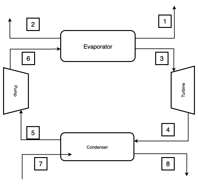
A geothermal Organic Rankine Cycle (ORC) system uses isobutane as the working fluid and water as the heating source. Hot water enters the evaporator at 158°C and 600 kPa, with a mass flow rate of 500 kg/s, and exits at a restricted temperature of 90°C. The working fluid, isobutane, evaporates at a pressure of 3250 kPa and condenses at 410 kPa. Cooling is provided by ambient air entering the condenser at 3°C with a mass flow rate of 8500 kg/s. You are required to model the thermodynamic performance of the cycle:
- Estimate the maximum isobutane flow rate based on heat availability,
- Turbine and pump work,
- Efficiency of the cycle
Solution:
First, we will set the known parameters
import ThermoSim
Model = ThermoSim.ThermodynamicModel()


T1 = 158+273.15 # Hot Water Inlet temperature
T2 = 90+273.15 # Hot water outlet
T3 = None
T4 = None
T5 = None
T6 = None
T7 = 3 + 273.15 # Air temperature
T8 = None


P1 = 6e5 #Hot Water Inlet Pressure
P2 = None
P3 = 3250e3 # Turbine Inlet Pressure
P4 = 410e3  # Turbine Outlet Pressure
P5 = None
P6 = None
P7 = 1.01e5 # Atmospheric Pressure
P8 = None


m_brine = 500
water = 'water'
w_fluid = 'Isobutane'
cooling_fluid = 'Air'
m_air = 8500
Now we make some assumptions and try to find other parameters.
#Assumptions
# No Pressure drop in HEX so
P2 = P1 # Eveporator: Hot side pressure of inlet and outlet is same
P5 = P4 # Eveporatore: cold side pressure of inlet and outlet is same
P6 = P3 # Condenser: Hot side pressure of inlet and outlet is same
P8 = P7 # Condenser: cold side pressure of inlet and outlet is same

# Consider 10K superheat for working fluid at evaporator outlet
T3 = Model.Prop(w_fluid, StatePointName = "demo", P = P3,Q = 1).T+10
# Consider 20K subcooling of working fluid at condenser outlet
T5 = Model.Prop(w_fluid,StatePointName="xxx",P = P5,Q = 0).T - 20

# Consider Pump and Turbines Isentropic efficiency
n_expn = .75
n_pump = 0.75
PPT = 5
Now we add the state points to our model.
Model.add_point(water, StatePointName = '1',P = P1, T = T1,Mass_flowrate=m_brine)
Model.add_point(water, StatePointName = '2',P = P2, T = T2)
Model.add_point(w_fluid, StatePointName = '3',P = P3, T = T3)
Model.add_point(w_fluid, StatePointName = '4',P = P4, T = T4)
Model.add_point(w_fluid, StatePointName = '5',P = P5, T = T5)
Model.add_point(w_fluid, StatePointName = '6',P = P6, T = T6)
Model.add_point(cooling_fluid, StatePointName = '7',P = P7, T = T7,Mass_flowrate=m_air)
Model.add_point(cooling_fluid, StatePointName = '8',P = P8, T = T8)
Model.Point_print()
Massflowrate of the working fluid is unknown so mass flowrate at state point 5 and 6 is set to 1 kg/s. It will show a warnig massage. As soon as we calculate the mass flowrate of the working fluid, we will recalculate the pump.
Pump = Model.Pump(Model, 'Pump', In_state = '5', Out_state = '6',n_isen=n_pump,Calculate=True)
Now solve the evaporator. Here, only missing paramtere is working fluids mass flow rate.
Evaporator = Model.HeatExchanger(Model, 'Evaporator', PPT = PPT, HEX_type = 'Evaporator', Hot_In_state = '1', Hot_Out_state = '2', Cold_In_state = '6', Cold_Out_state = '3',Calculate=True,PPT_graph=True)
As we know the mass flow rate of the working fluid, we recalculate the pump for accurate power of the pump.
Pump.Cal()
Now we solve the turbine and the condenser.
Turbine = Model.Turbine(Model, 'Turbine', In_state = '3', Out_state = '4',n_isen=n_expn,Calculate=True)


Condenser =  Model.HeatExchanger(Model, 'Condenser', PPT = PPT, HEX_type = 'Condenser', Hot_In_state = '4', Hot_Out_state = '5', Cold_In_state = '7', Cold_Out_state = '8',Calculate=True,PPT_graph=True)
Model.Point_print()
You can print all the component and state point by using the following command.
print(Model)
Now we can calculate and print the required parameters
working_fluid_massflowrate = Evaporator.Cold_Mass_flowrate
Turbine_work = Turbine.work
Pump_work = Pump.work
Q_in = Evaporator.Q
ORC_efficiency = (Turbine_work-Pump_work)/Q_in*100

print(f"Working Fluid's Mass Flowrate: {working_fluid_massflowrate} kg/s")
print(f"Turbine Power: {Turbine_work} W\n"
      f"Pump Power: {Pump_work} W")
print(f"Cycle Efficiency: {ORC_efficiency} %")
Tips
- You can add this
Model.Point_print()after every component to fidn which state point is solved.
License
MIT
Release history Release notifications | RSS feed


Download files
Download the file for your platform. If you're not sure which to choose, learn more about installing packages.
Source Distribution
Built Distribution
Filter files by name, interpreter, ABI, and platform.
If you're not sure about the file name format, learn more about wheel file names.
Copy a direct link to the current filters
File details
Details for the file thermosim-2.3.4.tar.gz.
File metadata
- Download URL: thermosim-2.3.4.tar.gz
- Upload date:
- Size: 43.6 kB
- Tags: Source
- Uploaded using Trusted Publishing? No
- Uploaded via: twine/6.1.0 CPython/3.13.3
File hashes
| Algorithm | Hash digest | |
|---|---|---|
| SHA256 |
b31f4f196eb683537ac97a57e0025c1cd836e1c4d56905f288dcebce84396a90
|
|
| MD5 |
c90c1fb18a0456ff8831cf06a0e48a13
|
|
| BLAKE2b-256 |
d7d4a613a7a12c6d77a018718e2e6ce14db709de8a3014bc0a973078b86a06be
|
File details
Details for the file thermosim-2.3.4-py3-none-any.whl.
File metadata
- Download URL: thermosim-2.3.4-py3-none-any.whl
- Upload date:
- Size: 23.5 kB
- Tags: Python 3
- Uploaded using Trusted Publishing? No
- Uploaded via: twine/6.1.0 CPython/3.13.3
File hashes
| Algorithm | Hash digest | |
|---|---|---|
| SHA256 |
634e4eeb11c5834f72ce0b9c8071b98b1bd1acee9b4a370fdc44ab412a50ae9d
|
|
| MD5 |
e36cd4acdde2c5cded461edd5e172f08
|
|
| BLAKE2b-256 |
3b40c37bdd0d556aec99337d44c15415d1737e25d2a239e934c1e789b74bf381
|


