Python Package for automated multivariate Time Series imputation

Project description


TimeWeaver: Automated time series imputation 
TimeWeaver is a Python library designed for multivariate time series data analysis, specifically addressing the challenges of machine process environmental data. It focuses on overcoming incomplete datasets due to sensor errors by employing various tailored imputation techniques. This ensures the integrity and relevance of data, catering to the unique characteristics of different features, such as discrepancies between power consumption and temperature curves.
TimeWeaver provides insightful graphics and analyses, enabling effective tool selection for specific data challenges, making it a valuable asset for data scientists and analysts. Additionally, it is evolving to offer a customizable Preprocessor model, facilitating the integration of optimal imputation methods into existing data processing pipelines for automated and enhanced data preparation.
Disclaimer
The currently implementation methods are based on the provided functions by numpy / scipy. The package logo was generated by ChatGPT 4.0 on 09.03.2024. The project is still in the early stages of development!
Quickstart
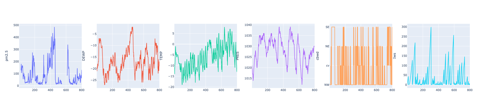
The following example uses the Beijing PM25 Data Set to show the functionalities of the library.
from timeweaver.timeweaver import TimeWeaver
from timeweaver.datasets import DataSets

dataframe = DataSets.PRSA()
interpolator = TimeWeaver(dataframe[0:1000], tracking_column="No")
interpolator.evaluate()
print(interpolator.get_best(optimized_selection=True))
[('year', 'akima'), ('month', 'akima'), ('day', 'akima'), ('hour', 'akima'), ('pm2.5', 'akima'), ('DEWP', 'from_derivatives'), ('TEMP', 'akima'), ('PRES', 'akima'), ('Iws', 'akima'), ('Is', 'from_derivatives'), ('Ir', 'akima')]
Structure
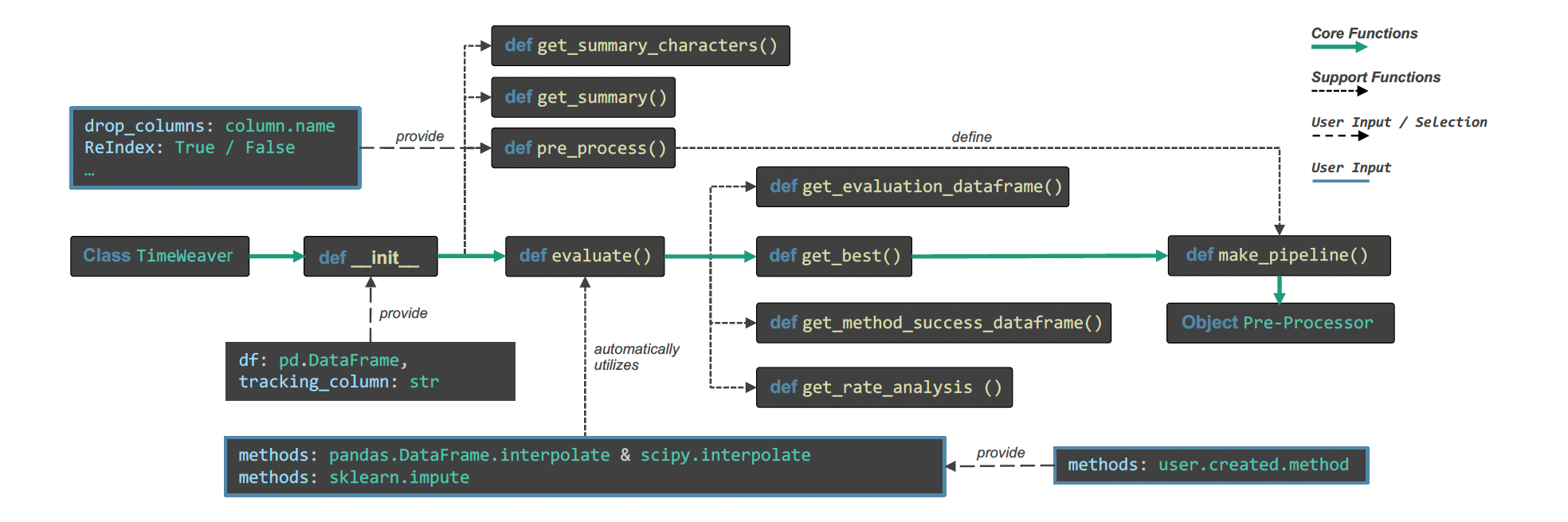
Functionalities
import pandas as pd
from timeweaver import TimeWeaver

dataframe = pd.read_csv("./src/data/PRSA/PRSA_data_2010.1.1-2014.12.31.csv")
dataframe
| No | year | month | day | hour | pm2.5 | DEWP | TEMP | PRES | cbwd | Iws | Is | Ir |
|---|---|---|---|---|---|---|---|---|---|---|---|---|
| 1 | 2010 | 1 | 1 | 0 | nan | -21 | -11 | 1021 | NW | 1.79 | 0 | 0 |
| 2 | 2010 | 1 | 1 | 1 | nan | -21 | -12 | 1020 | NW | 4.92 | 0 | 0 |
| 3 | 2010 | 1 | 1 | 2 | nan | -21 | -11 | 1019 | NW | 6.71 | 0 | 0 |
| 4 | 2010 | 1 | 1 | 3 | nan | -21 | -14 | 1019 | NW | 9.84 | 0 | 0 |
| 5 | 2010 | 1 | 1 | 4 | nan | -20 | -12 | 1018 | NW | 12.97 | 0 | 0 |
Initialize the TimeWeaver object and provide the dataframe and the tracking colum (Time or Index)
interpolator = TimeWeaver(dataframe[0:1000], tracking_column="No")
.get_summary() provides an general overview over the data. In this case we can identify that within the dataframe the features "pm2.5" utilizes NaNs and the "cbwd" is entirely consiting of non-numeric values.
interpolator.get_summary()
| Column | Data Type | Total Numeric Cells | Total Non-Numeric Cells | Total NaNs | Total Zero Values |
|---|---|---|---|---|---|
| No | int64 | 1000 | 0 | 0 | 0 |
| year | int64 | 1000 | 0 | 0 | 0 |
| month | int64 | 1000 | 0 | 0 | 0 |
| day | int64 | 1000 | 0 | 0 | 0 |
| hour | int64 | 1000 | 0 | 0 | 42 |
| pm2.5 | float64 | 909 | 0 | 91 | 0 |
| DEWP | int64 | 1000 | 0 | 0 | 0 |
| TEMP | float64 | 1000 | 0 | 0 | 48 |
| PRES | float64 | 1000 | 0 | 0 | 0 |
| cbwd | object | 0 | 1000 | 0 | 0 |
| Iws | float64 | 1000 | 0 | 0 | 0 |
| Is | int64 | 1000 | 0 | 0 | 958 |
| Ir | int64 | 1000 | 0 | 0 | 1000 |
.get_summary(full_summary=True) provides an more detailed overview.
interpolator.get_summary(full_summary=True)
| Column | Data Type | Total Numeric Cells | Total Non-Numeric Cells | Total NaNs | Total Zero Values | Unique Values Count | Most Frequent Value | Minimum Value | Maximum Value | Mean | Median |
|---|---|---|---|---|---|---|---|---|---|---|---|
| No | int64 | 1000 | 0 | 0 | 0 | 1000 | 1 | 1 | 1000 | 500.5 | 500.5 |
| year | int64 | 1000 | 0 | 0 | 0 | 1 | 2010 | 2010 | 2010 | 2010 | 2010 |
| month | int64 | 1000 | 0 | 0 | 0 | 2 | 1 | 1 | 2 | 1.256 | 1 |
| day | int64 | 1000 | 0 | 0 | 0 | 31 | 1 | 1 | 31 | 13.4 | 11 |
| hour | int64 | 1000 | 0 | 0 | 42 | 24 | 0 | 0 | 23 | 11.436 | 11 |
| pm2.5 | float64 | 909 | 0 | 91 | 0 | 257 | 27.0 | 6 | 485 | 88.363 | 61 |
| DEWP | int64 | 1000 | 0 | 0 | 0 | 26 | -19 | -27 | -2 | -16.269 | -17 |
| TEMP | float64 | 1000 | 0 | 0 | 48 | 28 | -5.0 | -19 | 8 | -5.483 | -5 |
| PRES | float64 | 1000 | 0 | 0 | 0 | 28 | 1027.0 | 1012 | 1039 | 1027.82 | 1028 |
| cbwd | object | 0 | 1000 | 0 | 0 | 4 | NW | nan | nan | nan | nan |
| Iws | float64 | 1000 | 0 | 0 | 0 | 398 | 0.89 | 0.45 | 299.06 | 34.1421 | 9.84 |
| Is | int64 | 1000 | 0 | 0 | 958 | 26 | 0 | 0 | 27 | 0.414 | 0 |
| Ir | int64 | 1000 | 0 | 0 | 1000 | 1 | 0 | 0 | 0 | 0 | 0 |
.get_summary_characters() provides insights into individual characters within the data.
interpolator.get_summary(full_summary=True)
| Column | Data Type | Total Non-Numeric | Total Numeric | n | a | . | - | N | W | c | v | E | S |
|---|---|---|---|---|---|---|---|---|---|---|---|---|---|
| No | int64 | 0 | 2893 | 0 | 0 | 0 | 0 | 0 | 0 | 0 | 0 | 0 | 0 |
| year | int64 | 0 | 4000 | 0 | 0 | 0 | 0 | 0 | 0 | 0 | 0 | 0 | 0 |
| month | int64 | 0 | 1000 | 0 | 0 | 0 | 0 | 0 | 0 | 0 | 0 | 0 | 0 |
| day | int64 | 0 | 1568 | 0 | 0 | 0 | 0 | 0 | 0 | 0 | 0 | 0 | 0 |
| hour | int64 | 0 | 1580 | 0 | 0 | 0 | 0 | 0 | 0 | 0 | 0 | 0 | 0 |
| pm2.5 | float64 | 1182 | 2982 | 182 | 91 | 909 | 0 | 0 | 0 | 0 | 0 | 0 | 0 |
| DEWP | int64 | 1000 | 1845 | 0 | 0 | 0 | 1000 | 0 | 0 | 0 | 0 | 0 | 0 |
| TEMP | float64 | 1821 | 2246 | 0 | 0 | 1000 | 821 | 0 | 0 | 0 | 0 | 0 | 0 |
| PRES | float64 | 1000 | 5000 | 0 | 0 | 1000 | 0 | 0 | 0 | 0 | 0 | 0 | 0 |
| cbwd | object | 2000 | 0 | 0 | 0 | 0 | 0 | 690 | 528 | 155 | 155 | 317 | 155 |
| Iws | float64 | 1000 | 3532 | 0 | 0 | 1000 | 0 | 0 | 0 | 0 | 0 | 0 | 0 |
| Is | int64 | 0 | 1017 | 0 | 0 | 0 | 0 | 0 | 0 | 0 | 0 | 0 | 0 |
| Ir | int64 | 0 | 1000 | 0 | 0 | 0 | 0 | 0 | 0 | 0 | 0 | 0 | 0 |
.evaluate() is the core function of TimeWeaver and tests the different methods on the dataframe.
interpolator.evaluate()
➤ Evaluation complete. ✔
➤ Evaluated number of methods: 21 ✔
If the evaluation is done the user can access differrent methods to retrieve the analysis resuslts and gain more insights into the imputation results.
results_df = interpolator.get_evaluation_dataframe()
results_df
| linear | nearest | zero | slinear | quadratic | ... | |
|---|---|---|---|---|---|---|
| year | 0 | 0 | 0 | 0 | 0 | |
| month | 0 | 0 | 0 | 0 | 0.0001 | |
| day | 0.045 | 0.07 | 0.06 | 0.045 | 0.0741 | |
| hour | 1.08 | 2.54 | 2.44 | 1.08 | 1.7227 | |
| pm2.5 | 10.412 | 13.1011 | 12.3483 | 10.412 | 10.6714 | |
| DEWP | 0.6783 | 0.88 | 0.86 | 0.6783 | 0.7843 | |
| TEMP | 0.72 | 1.03 | 1.17 | 0.72 | 0.8513 | |
| PRES | 0.395 | 0.55 | 0.53 | 0.395 | 0.4227 | |
| cbwd | nan | nan | nan | nan | nan | |
| Iws | 2.972 | 6.2409 | 5.6463 | 2.972 | 4.3372 | |
| Is | 0.025 | 0.09 | 0.09 | 0.025 | 0.0352 | |
| Ir | 0 | 0 | 0 | 0 | 0 |
results_df = interpolator.get_method_success_dataframe()
results_df
| linear | nearest | zero | slinear | quadratic | ... | |
|---|---|---|---|---|---|---|
| year | 1 | 1 | 1 | 1 | 1 | |
| month | 1 | 1 | 1 | 1 | 1 | |
| day | 1 | 1 | 1 | 1 | 1 | |
| hour | 1 | 1 | 1 | 1 | 1 | |
| pm2.5 | 1 | 1 | 1 | 1 | 1 | |
| DEWP | 1 | 1 | 1 | 1 | 1 | |
| TEMP | 1 | 1 | 1 | 1 | 1 | |
| PRES | 1 | 1 | 1 | 1 | 1 | |
| cbwd | 0 | 0 | 0 | 0 | 0 | |
| Iws | 1 | 1 | 1 | 1 | 1 | |
| Is | 1 | 1 | 1 | 1 | 1 | |
| Ir | 1 | 1 | 1 | 1 | 1 |
results_df = interpolator.get_best(optimized_selection=False)
results_df
{'year': ['linear', 'nearest', 'zero', 'slinear', 'quadratic', 'cubic', 'polynomial_order_1', 'polynomial_order_2', 'polynomial_order_3', 'polynomial_order_5', 'polynomial_order_7', 'polynomial_order_9', 'piecewise_polynomial', 'spline_order_1', 'spline_order_2', 'spline_order_3', 'spline_order_4', 'spline_order_5', 'akima', 'cubicspline', 'from_derivatives'], 'month': ['linear', 'nearest', 'zero', 'slinear', 'polynomial_order_1', 'piecewise_polynomial', 'akima', 'from_derivatives'], 'day': ['linear', 'slinear', 'polynomial_order_1', 'piecewise_polynomial', 'akima', 'from_derivatives'], 'hour': ['linear', 'slinear', 'polynomial_order_1', 'piecewise_polynomial', 'akima', 'from_derivatives'], 'pm2.5': ['akima'], 'DEWP': ['linear', 'slinear', 'polynomial_order_1', 'piecewise_polynomial', 'from_derivatives'], 'TEMP': ['akima'], 'PRES': ['akima'], 'cbwd': [], 'Iws': ['akima'], 'Is': ['linear', 'slinear', 'polynomial_order_1', 'piecewise_polynomial', 'from_derivatives'], 'Ir': ['linear', 'nearest', 'zero', 'slinear', 'quadratic', 'cubic', 'polynomial_order_1', 'polynomial_order_2', 'polynomial_order_3', 'polynomial_order_5', 'polynomial_order_7', 'polynomial_order_9', 'piecewise_polynomial', 'spline_order_1', 'spline_order_2', 'spline_order_3', 'spline_order_4', 'spline_order_5', 'akima', 'cubicspline', 'from_derivatives']}
results_df = interpolator.get_best(optimized_selection=True)
results_df
[('year', 'akima'), ('month', 'akima'), ('day', 'akima'), ('hour', 'akima'), ('pm2.5', 'akima'), ('DEWP', 'from_derivatives'), ('TEMP', 'akima'), ('PRES', 'akima'), ('Iws', 'akima'), ('Is', 'from_derivatives'), ('Ir', 'akima')]
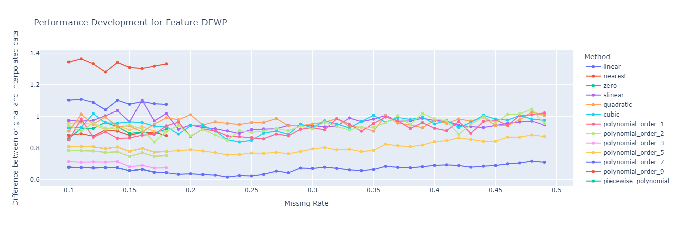
interpolator.get_rate_analysis()
Release history Release notifications | RSS feed


Download files
Download the file for your platform. If you're not sure which to choose, learn more about installing packages.
Source Distribution
File details
Details for the file TimeWeaver-0.1.7.24.tar.gz.
File metadata
- Download URL: TimeWeaver-0.1.7.24.tar.gz
- Upload date:
- Size: 518.7 kB
- Tags: Source
- Uploaded using Trusted Publishing? No
- Uploaded via: twine/5.0.0 CPython/3.8.18
File hashes
| Algorithm | Hash digest | |
|---|---|---|
| SHA256 |
4a4b40d20725fac678bce5e988fbb76f0d2e4a06c69f89503475f7afb706e4ad
|
|
| MD5 |
37d75e63ac2da8440fbe752cc6e33d12
|
|
| BLAKE2b-256 |
596168a02b2e73aba3981257d73b082f85b6804aeb6bdb02a4c64ef0d6981b11
|


