
MCMC tools for astrophysics

Project description
VegasAfterglow








VegasAfterglow is a high-performance C++ framework with a user-friendly Python interface designed for the comprehensive modeling of afterglows. It achieves exceptional computational efficiency, enabling the generation of multi-wavelength light curves in milliseconds and facilitating robust Markov Chain Monte Carlo (MCMC) parameter inference in seconds to minutes. The framework incorporates advanced models for shock dynamics (both forward and reverse shocks), diverse radiation mechanisms (synchrotron with self-absorption, and inverse Compton scattering with Klein-Nishina corrections), and complex structured jet configurations. For lightweight afterglow modeling, one can also consider the PyFRS package.
Table of Contents
Features
Shock Dynamics
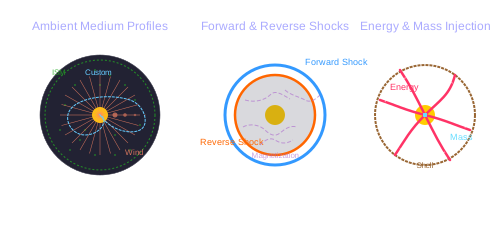
- Forward and Reverse Shock Modeling: Simulates both shocks via shock crossing dynamics with arbitrary magnetization levels and shell thicknesses.
- Relativistic and Non-Relativistic Regimes: Accurately models shock evolution across all velocity regimes.
- Adiabatic and Radiative Blast Waves: Supports smooth transition between adiabatic and radiative blast waves.
- Ambient Medium: Supports uniform Interstellar Medium (ISM), stellar wind environments, and user-defined density profiles.
- Energy and Mass Injection: Supports user-defined profiles for continuous energy and/or mass injection into the blast wave.
Jet Structure & Geometry
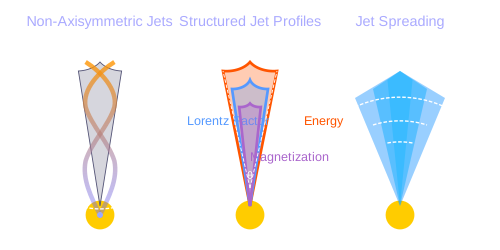
- Structured Jet Profiles: Allows user-defined angular profiles for energy distribution, initial Lorentz factor, and magnetization.
- Arbitrary Viewing Angles: Supports off-axis observers at any viewing angle relative to the jet axis.
- Jet Spreading: Includes lateral expansion dynamics for realistic jet evolution (experimental).
- Non-Axisymmetric Jets: Capable of modeling complex, non-axisymmetric jet structures.
Radiation Mechanisms
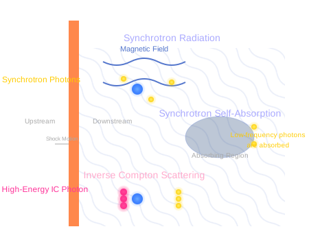
- Synchrotron Radiation: Calculates synchrotron emission from shocked electrons.
- Synchrotron Self-Absorption (SSA): Includes SSA effects, crucial at low frequencies.
- Inverse Compton (IC) Scattering: Models IC processes, including:
- Synchrotron Self-Compton (SSC) from both forward and reverse shocks.
- Pairwise IC between forward and reverse shock electron and photon populations (experimental).
- Includes Klein-Nishina corrections for accurate synchrotron and IC emission.
Performance Highlights
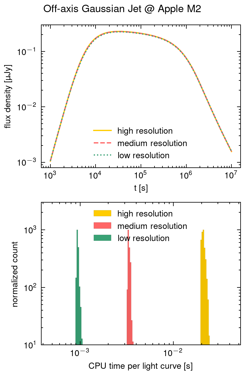
VegasAfterglow delivers exceptional computational performance through deep optimization of its core algorithms:
-
Ultra-fast Light Curve Computation: Generates a 100-point single-frequency light curve (forward shock & synchrotron only) from a structured jet viewed off-axis in approximately 1 millisecond on an Apple M2 chip with a single core.
-
Rapid MCMC Exploration: Enables parameter estimation with 10,000 MCMC steps for 8 parameters on 20 data points across multi-wavelength light curves and spectra on an 8-core Apple M2 chip in:
- ~50 seconds for on-axis structured jet scenarios
This level of performance is achieved through optimized algorithm implementation and efficient memory access patterns, facilitating comprehensive Bayesian inference on standard laptop hardware in seconds to minutes rather than hours or days. The accelerated convergence speed enables rapid iteration through different physical models and makes VegasAfterglow suitable for both detailed analysis of individual GRB events and large-scale population studies.
Installation
VegasAfterglow is available as a Python package with C++ source code also provided for direct use.
Python Installation
To install VegasAfterglow using pip:
pip install VegasAfterglow
This is the recommended method for most users. VegasAfterglow requires Python 3.8 or higher.
Alternative: Install from Source (click to expand/collapse)
For cases where pip installation is not viable or when the development version is required:
- Clone this repository:
git clone https://github.com/YihanWangAstro/VegasAfterglow.git
- Navigate to the directory and install the Python package:
cd VegasAfterglow
pip install .
Standard development environments typically include the necessary prerequisites (C++20 compatible compiler). For build-related issues, refer to the prerequisites section in C++ Installation.
C++ Installation
For advanced users who need to compile and use the C++ library directly:
Instructions for C++ Installation (click to expand/collapse)
- Clone the repository (if not previously done):
git clone https://github.com/YihanWangAstro/VegasAfterglow.git
cd VegasAfterglow
- Compile and run tests:
make tests
Upon successful compilation, you can create custom C++ problem generators using the VegasAfterglow interfaces. For implementation details, refer to the Creating Custom Problem Generators with C++ section or examine the example problem generators in tests/demo/.
Build Prerequisites (click to expand for dependency information)
The following development tools are required:
-
C++20 compatible compiler:
- Linux: GCC 10+ or Clang 13+
- macOS: Apple Clang 13+ (with Xcode 13+) or GCC 10+ (via Homebrew)
- Windows: MSVC 19.29+ (Visual Studio 2019 16.10+) or MinGW-w64 with GCC 10+
-
Build tools:
- Make (GNU Make 4.0+ recommended)
Usage
Quick Start
We provide basic example scripts (script/quick.ipynb, script/details.ipynb and script/mcmc.ipynb) that demonstrate how to set up and run afterglow simulations. This section shows how to calculate light curves and spectra for a simple GRB afterglow model without the need for observational data and perform MCMC parameter fitting with observational data. The notebook can be run using either Jupyter Notebook or VSCode with the Jupyter extension.
To avoid conflicts when updating the repository in the future, make a copy of the example notebook in the same directory and work with the copy instead of the original.
Light Curve & Spectrum Calculation
The example below walks through the main components needed to model a GRB afterglow, from setting up the physical parameters to producing light curves and spectra via script/quick.ipynb.
Model Setup (click to expand/collapse)
First, let's set up the physical components of our afterglow model, including the environment, jet, observer, and radiation parameters:
import numpy as np
import matplotlib.pyplot as plt
from VegasAfterglow import ISM, TophatJet, Observer, Radiation, Model

# 1. Define the circumburst environment (constant density ISM)
medium = ISM(n_ism=1) #in cgs unit

# 2. Configure the jet structure (top-hat with opening angle, energy, and Lorentz factor)
jet = TophatJet(theta_c=0.1, E_iso=1e52, Gamma0=300) #in cgs unit

# 3. Set observer parameters (distance, redshift, viewing angle)
obs = Observer(lumi_dist=1e26, z=0.1, theta_obs=0) #in cgs unit

# 4. Define radiation microphysics parameters
rad = Radiation(eps_e=1e-1, eps_B=1e-3, p=2.3)

# 5. Combine all components into a complete afterglow model
model = Model(jet=jet, medium=medium, observer=obs, fwd_rad=rad)
Light Curve Calculation (click to expand/collapse)
Now, let's compute and plot multi-wavelength light curves to see how the afterglow evolves over time:
# 1. Create logarithmic time array from 10² to 10⁸ seconds (100s to ~3yrs)
times = np.logspace(2, 8, 100)

# 2. Define observing frequencies (radio, optical, X-ray bands in Hz)
bands = np.array([1e9, 1e14, 1e17])

# 3. Calculate the afterglow emission at each time and frequency
# NOTE: times array must be in ascending order, frequencies can be in random order
results = model.flux_density_grid(times, bands)

# 4. Visualize the multi-wavelength light curves
plt.figure(figsize=(4.8, 3.6),dpi=200)

# 5. Plot each frequency band
for i, nu in enumerate(bands):
    exp = int(np.floor(np.log10(nu)))
    base = nu / 10**exp
    plt.loglog(times, results.total[i,:], label=fr'${base:.1f} \times 10^{{{exp}}}$ Hz')

def add_note(plt):
    plt.annotate('jet break',xy=(3e4, 1e-26), xytext=(3e3, 5e-28), arrowprops=dict(arrowstyle='->'))
    plt.annotate(r'$\nu_m=\nu_a$',xy=(8e5, 2e-25), xytext=(7.5e4, 5e-24), arrowprops=dict(arrowstyle='->'))
    plt.annotate(r'$\nu=\nu_a$',xy=(4e6, 4e-25), xytext=(7.5e5, 5e-24), arrowprops=dict(arrowstyle='->'))

add_note(plt)
plt.xlabel('Time (s)')
plt.ylabel('Flux Density (erg/cm²/s/Hz)')
plt.legend()
plt.title('Light Curves')
plt.savefig('quick-lc.png',dpi=300,bbox_inches='tight')

Running the light curve script will produce this figure showing the afterglow evolution across different frequencies.
Spectrum Analysis (click to expand/collapse)
We can also examine how the broadband spectrum evolves at different times after the burst:
# 1. Define broad frequency range (10⁵ to 10²² Hz)
frequencies = np.logspace(5, 22, 100)

# 2. Select specific time epochs for spectral snapshots
epochs = np.array([1e2, 1e3, 1e4, 1e5 ,1e6, 1e7, 1e8])

# 3. Calculate spectra at each epoch
# NOTE: epochs array must be in ascending order, frequencies can be in random order
results = model.flux_density_grid(epochs, frequencies)

# 4. Plot broadband spectra at each epoch
plt.figure(figsize=(4.8, 3.6),dpi=200)
colors = plt.cm.viridis(np.linspace(0,1,len(epochs)))

for i, t in enumerate(epochs):
    exp = int(np.floor(np.log10(t)))
    base = t / 10**exp
    plt.loglog(frequencies, results.total[:,i], color=colors[i], label=fr'${base:.1f} \times 10^{{{exp}}}$ s')

# 5. Add vertical lines marking the bands from the light curve plot
for i, band in enumerate(bands):
    exp = int(np.floor(np.log10(band)))
    base = band / 10**exp
    plt.axvline(band,ls='--',color='C'+str(i))

plt.xlabel('frequency (Hz)')
plt.ylabel('flux density (erg/cm²/s/Hz)')
plt.legend(ncol=2)
plt.title('Synchrotron Spectra')
plt.savefig('quick-spec.png',dpi=300,bbox_inches='tight')

The spectral analysis code will generate this visualization showing spectra at different times, with vertical lines indicating the frequencies calculated in the light curve example.
Time-Frequency Pairs Calculation (click to expand/collapse)
If you want to calculate flux at specific time-frequency pairs (t_i, nu_i) instead of a grid (t_i, nu_j), you can use the alternative series interfaces:
# Define time and frequency arrays (must be the same length)
times = np.logspace(2, 8, 200)
frequencies = np.logspace(9, 17, 200)

# For time-frequency pairs (times array must be in ascending order)
results = model.flux_density(times, frequencies)

# The returned results is a FluxDict object with different flux components
print("Result attributes:", dir(results))  # Shows .fwd, .rvs, .total attributes
print("Total flux shape:", results.total.shape)  # Same shape as input arrays
print("Forward shock shape:", results.fwd.sync.shape)  # Forward shock synchrotron component
Key differences:
flux_density_grid(): Calculates flux on a time-frequency grid (NxM output from N times and M frequencies)flux_density(): Calculates flux at paired time-frequency points (N output from N time-frequency pairs), requires ascending order time arraysflux_density_exposures(): Same as above but with exposure time averaging for realistic observational scenarios
Return value structure:
All flux calculation methods return a FluxDict object with:
.total: Combined flux from all components.fwd: Forward shock flux (has.syncand.sscattributes).rvs: Reverse shock flux (has.syncand.sscattributes)
Internal Quantities Evolution
The example below walks through how you can check the evolution of internal quantities under various reference frames via script/details.ipynb.
Model Setup (click to expand/collapse)
Same as for light curve generation, let's set up the physical components of our afterglow model, including the environment, jet, observer, and radiation parameters:
import numpy as np
import matplotlib.pyplot as plt
from VegasAfterglow import ISM, TophatJet, Observer, Radiation, Model

medium = ISM(n_ism=1)

jet = TophatJet(theta_c=0.3, E_iso=1e52, Gamma0=100)

obs = Observer(lumi_dist=1e26, z=0.1, theta_obs=0.)

rad = Radiation(eps_e=1e-1, eps_B=1e-3, p=2.3)

model = Model(jet=jet, medium=medium, observer=obs, fwd_rad=rad, resolutions=(0.1,5,10))
Get the simulation quantities (click to expand/collapse)
Now, let's get the internal simulation quantities:
# Get the simulation details over a time range
details = model.details(t_min=1e0, t_max=1e8)

# Print the available attributes
print("Simulation details attributes:", dir(details))
print("Forward shock attributes:", dir(details.fwd))
You will get a SimulationDetails object with the following structure:
Main grid coordinates:
details.phi: 1D numpy array of azimuthal angles inradiansdetails.theta: 1D numpy array of polar angles inradiansdetails.t_src: 3D numpy array of source frame times on coordinate (phi_i, theta_j, t_k) grid inseconds
Forward shock details (accessed via details.fwd):
details.fwd.t_comv: 3D numpy array of comoving times for the forward shock insecondsdetails.fwd.t_obs: 3D numpy array of observer times for the forward shock insecondsdetails.fwd.Gamma: 3D numpy array of downstream Lorentz factors for the forward shockdetails.fwd.Gamma_th: 3D numpy array of thermal Lorentz factors for the forward shockdetails.fwd.r: 3D numpy array of lab frame radii incmdetails.fwd.B_comv: 3D numpy array of downstream comoving magnetic field strengths for the forward shock inGaussdetails.fwd.theta: 3D numpy array of polar angles for the forward shock inradiansdetails.fwd.N_p: 3D numpy array of downstream shocked proton number per solid angle for the forward shockdetails.fwd.N_e: 3D numpy array of downstream synchrotron electron number per solid angle for the forward shockdetails.fwd.gamma_a: 3D numpy array of comoving frame self-absorption Lorentz factors for the forward shockdetails.fwd.gamma_m: 3D numpy array of comoving frame injection Lorentz factors for the forward shockdetails.fwd.gamma_c: 3D numpy array of comoving frame cooling Lorentz factors for the forward shockdetails.fwd.gamma_M: 3D numpy array of comoving frame maximum Lorentz factors for the forward shockdetails.fwd.nu_a: 3D numpy array of comoving frame self-absorption frequencies for the forward shock inHzdetails.fwd.nu_m: 3D numpy array of comoving frame injection frequencies for the forward shock inHzdetails.fwd.nu_c: 3D numpy array of comoving frame cooling frequencies for the forward shock inHzdetails.fwd.nu_M: 3D numpy array of comoving frame maximum frequencies for the forward shock inHzdetails.fwd.I_nu_max: 3D numpy array of comoving frame synchrotron maximum specific intensities for the forward shock inerg/cm²/s/Hzdetails.fwd.Doppler: 3D numpy array of Doppler factors for the forward shock
Reverse shock details (accessed via details.rvs, if reverse shock is enabled):
- Similar attributes as forward shock but for the reverse shock component
Checking the evolution of various parameters (click to expand/collapse)
To analyze the temporal evolution of physical parameters across different reference frames, we can visualize how key quantities evolve in the source, comoving, and observer frames. The following analysis demonstrates the comprehensive tracking of shock dynamics and microphysical parameters throughout the afterglow evolution:
Multi-parameter evolution visualization: This code creates a comprehensive multi-panel figure displaying the temporal evolution of fundamental shock parameters (Lorentz factor, magnetic field, particle numbers, radius, and peak synchrotron power) across all three reference frames:
attrs =['Gamma', 'B_comv', 'N_p','r','N_e','I_nu_max']
ylabels = [r'$\Gamma$', r'$B^\prime$ [G]', r'$N_p$', r'$r$ [cm]', r'$N_e$', r'$I_{\nu, \rm max}^\prime$ [erg/s/Hz]']

frames = ['t_src', 't_comv', 't_obs']
titles = ['source frame', 'comoving frame', 'observer frame']
colors = ['C0', 'C1', 'C2']
xlabels = [r'$t_{\rm src}$ [s]', r'$t^\prime$ [s]', r'$t_{\rm obs}$ [s]']
plt.figure(figsize= (4.2*len(frames), 3*len(attrs)))

#plot the evolution of various parameters for phi = 0 and theta = 0 (so the first two indexes are 0)
for i, frame in enumerate(frames):
    for j, attr in enumerate(attrs):
        plt.subplot(len(attrs), len(frames) , j * len(frames) + i + 1)
        if j == 0:
            plt.title(titles[i])
        value = getattr(details.fwd, attr)
        if frame == 't_src':
            t = getattr(details, frame)
        else:
            t = getattr(details.fwd, frame)
        plt.loglog(t[0, 0, :], value[0, 0, :], color='k',lw=2.5)
        plt.loglog(t[0, 0, :], value[0, 0, :], color=colors[i])

        plt.xlabel(xlabels[i])
        plt.ylabel(ylabels[j])

plt.tight_layout()
plt.savefig('shock_quantities.png', dpi=300,bbox_inches='tight')

Electron energy distribution analysis: This visualization focuses specifically on the characteristic electron energies (self-absorption, injection, and cooling) across all three reference frames:
frames = ['t_src', 't_comv', 't_obs']
xlabels = [r'$t_{\rm src}$ [s]', r'$t^\prime$ [s]', r'$t_{\rm obs}$ [s]']
plt.figure(figsize= (4.2*len(frames), 3.6))

for i, frame in enumerate(frames):
    plt.subplot(1, len(frames), i + 1)
    if frame == 't_src':
        t = getattr(details, frame)
    else:
        t = getattr(details.fwd, frame)
    plt.loglog(t[0, 0, :], details.fwd.gamma_a[0, 0, :],label=r'$\gamma_a^\prime$',c='firebrick')
    plt.loglog(t[0, 0, :], details.fwd.gamma_m[0, 0, :],label=r'$\gamma_m^\prime$',c='yellowgreen')
    plt.loglog(t[0, 0, :], details.fwd.gamma_c[0, 0, :],label=r'$\gamma_c^\prime$',c='royalblue')
    plt.loglog(t[0, 0, :], details.fwd.gamma_a[0, 0, :]*details.fwd.Doppler[0,0,:],label=r'$\gamma_a$',ls='--',c='firebrick')
    plt.loglog(t[0, 0, :], details.fwd.gamma_m[0, 0, :]*details.fwd.Doppler[0,0,:],label=r'$\gamma_m$',ls='--',c='yellowgreen')
    plt.loglog(t[0, 0, :], details.fwd.gamma_c[0, 0, :]*details.fwd.Doppler[0,0,:],label=r'$\gamma_c$',ls='--',c='royalblue')
    plt.xlabel(xlabels[i])
    plt.ylabel(r'$\gamma_e^\prime$')
    plt.legend(ncol=2)
plt.tight_layout()
plt.savefig('electron_quantities.png', dpi=300,bbox_inches='tight')

Synchrotron frequency evolution: This analysis tracks the evolution of characteristic synchrotron frequencies:
frames = ['t_src', 't_comv', 't_obs']
xlabels = [r'$t_{\rm src}$ [s]', r'$t^\prime$ [s]', r'$t_{\rm obs}$ [s]']
plt.figure(figsize= (4.2*len(frames), 3.6))

for i, frame in enumerate(frames):
    plt.subplot(1, len(frames), i + 1)
    if frame == 't_src':
        t = getattr(details, frame)
    else:
        t = getattr(details.fwd, frame)
    plt.loglog(t[0, 0, :], details.fwd.nu_a[0, 0, :],label=r'$\nu_a^\prime$',c='firebrick')
    plt.loglog(t[0, 0, :], details.fwd.nu_m[0, 0, :],label=r'$\nu_m^\prime$',c='yellowgreen')
    plt.loglog(t[0, 0, :], details.fwd.nu_c[0, 0, :],label=r'$\nu_c^\prime$',c='royalblue')
    plt.loglog(t[0, 0, :], details.fwd.nu_a[0, 0, :]*details.fwd.Doppler[0,0,:],label=r'$\nu_a$',ls='--',c='firebrick')
    plt.loglog(t[0, 0, :], details.fwd.nu_m[0, 0, :]*details.fwd.Doppler[0,0,:],label=r'$\nu_m$',ls='--',c='yellowgreen')
    plt.loglog(t[0, 0, :], details.fwd.nu_c[0, 0, :]*details.fwd.Doppler[0,0,:],label=r'$\nu_c$',ls='--',c='royalblue')
    plt.xlabel(xlabels[i])
    plt.ylabel(r'$\nu$ [Hz]')
    plt.legend(ncol=2)
plt.tight_layout()
plt.savefig('photon_quantities.png', dpi=300,bbox_inches='tight')

Doppler factor spatial distribution: This polar plot visualizes the spatial distribution of the Doppler factor across the jet structure, showing how relativistic beaming varies with angular position and radial distance:
plt.figure(figsize=(6,6))
ax = plt.subplot(111, polar=True)

theta = details.fwd.theta[0,:,:]
r     = details.fwd.r[0,:,:]
D     = details.fwd.Doppler[0,:,:]

# Polar contour plot
scale = 3.0
c = ax.contourf(theta*scale, r, np.log10(D), levels=30, cmap='viridis')

ax.set_rscale('log')
true_ticks = np.linspace(0, 0.3, 6)
ax.set_xticks(true_ticks * scale)
ax.set_xticklabels([f"{t:.2f}" for t in true_ticks])
ax.set_xlim(0,0.3*scale)
ax.set_ylabel(r'$\theta$ [rad]')
ax.set_xlabel(r'$r$ [cm]')

plt.colorbar(c, ax=ax, label=r'$\log_{10} D$')

plt.tight_layout()
plt.savefig('doppler.png', dpi=300,bbox_inches='tight')

Equal arrival time (EAT) surface visualization: This final visualization maps the equal arrival time surfaces in polar coordinates, illustrating how light from different parts of the jet reaches the observer at the same time:
plt.figure(figsize=(6,6))
ax = plt.subplot(111, polar=True)

theta = details.fwd.theta[0,:,:]
r     = details.fwd.r[0,:,:]
t_obs = details.fwd.t_obs[0,:,:]

scale = 3.0
c = ax.contourf(theta*scale, r, np.log10(t_obs), levels=30, cmap='viridis')

ax.set_rscale('log')
true_ticks = np.linspace(0, 0.3, 6)
ax.set_xticks(true_ticks * scale)
ax.set_xticklabels([f"{t:.2f}" for t in true_ticks])
ax.set_xlim(0,0.3*scale)
ax.set_ylabel(r'$\theta$ [rad]')
ax.set_xlabel(r'$r$ [cm]')

plt.colorbar(c, ax=ax, label=r'$\log_{10} (t_{\rm obs}/s)$')

plt.tight_layout()
plt.savefig('EAT.png', dpi=300,bbox_inches='tight')

MCMC Parameter Fitting
We provide some example data files in the data folder. Remember to keep your copy in the same directory as the original to ensure all data paths work correctly.
1. Preparing Data and Configuring the Model (click to expand/collapse)
import numpy as np
import matplotlib.pyplot as plt
import pandas as pd
import corner
from VegasAfterglow import ObsData, Setups, Fitter, ParamDef, Scale
VegasAfterglow provides flexible options for loading observational data through the ObsData class. You can add light curves (specific flux vs. time) and spectra (specific flux vs. frequency) in multiple ways.
# Create an instance to store observational data
data = ObsData()

# Method 1: Add data directly from lists or numpy arrays

# For light curves
t_data = [1e3, 2e3, 5e3, 1e4, 2e4]  # Time in seconds
flux_data = [1e-26, 8e-27, 5e-27, 3e-27, 2e-27]  # Specific flux in erg/cm²/s/Hz
flux_err = [1e-28, 8e-28, 5e-28, 3e-28, 2e-28]  # Specific flux error in erg/cm²/s/Hz
data.add_flux_density(nu=4.84e14, t=t_data, f_nu=flux_data, err=flux_err)  # All quantities in CGS units
# You can also assign weights to each data point to account for systematic uncertainties or correlations. You don't need to worry about the weights' normalization, the code will normalize them automatically.
#data.add_flux_density(nu=4.84e14, t=t_data, f_nu=flux_data, err=flux_err, weights=np.ones(len(t_data)))

# For spectra
nu_data = [...]  # Frequencies in Hz
spectrum_data = [...] # Specific flux values in erg/cm²/s/Hz
spectrum_err = [...]   # Specific flux errors in erg/cm²/s/Hz
data.add_spectrum(t=3000, nu=nu_data, f_nu=spectrum_data, err=spectrum_err, weights=np.ones(len(nu_data)))  # All quantities in CGS units
# Method 2: Load from CSV files

data = ObsData()
# Define your bands and files
bands = [2.4e17, 4.84e14, 1.4e14]  # Example: X-ray, optical R-band
lc_files = ["data/ep.csv", "data/r.csv", "data/vt-r.csv"]

# Load light curves from files
for nu, fname in zip(bands, lc_files):
    df = pd.read_csv(fname)
    data.add_flux_density(nu=nu, t=df["t"], f_nu=df["Fv_obs"], err=df["Fv_err"])  # All quantities in CGS units

times = [3000] # Example: time in seconds
spec_files = ["data/ep-spec.csv"]

# Load spectra from files
for t, fname in zip(times, spec_files):
    df = pd.read_csv(fname)
    data.add_spectrum(t=t, nu=df["nu"], f_nu=df["Fv_obs"], err=df["Fv_err"])  # All quantities in CGS units
Note: The
ObsDatainterface is designed to be flexible. You can mix and match different data sources, and add multiple light curves at different frequencies as well as multiple spectra at different times.
The Setups class defines the global properties and environment for your model. These settings remain fixed during the MCMC process. Check the documentation for all available options.
cfg = Setups()

# Source properties
cfg.lumi_dist = 3.364e28    # Luminosity distance [cm]
cfg.z = 1.58               # Redshift

# Physical model configuration
cfg.medium = "wind"        # Ambient medium: "wind", "ism", etc. (see documentation)
cfg.jet = "powerlaw"       # Jet structure: "powerlaw", "gaussian", "tophat", etc. (see documentation)
These settings affect how the model is calculated but are not varied during the MCMC process.
2. Defining Parameters and Running MCMC (click to expand/collapse)
The ParamDef class is used to define the parameters for MCMC exploration. Each parameter requires a name, prior range, and sampling scale:
mc_params = [
    ParamDef("E_iso",      1e50,  1e54,  Scale.LOG),       # Isotropic energy [erg]
    ParamDef("Gamma0",        5,  1000,  Scale.LOG),       # Lorentz factor at the core
    ParamDef("theta_c",     0.0,   0.5,  Scale.LINEAR),    # Core half-opening angle [rad]
    ParamDef("k_e",           2,     2,  Scale.FIXED),     # Energy power law index
    ParamDef("k_g",           2,     2,  Scale.FIXED),     # Lorentz factor power law index
    ParamDef("theta_v",     0.0,   0.0,  Scale.FIXED),     # Viewing angle [rad]
    ParamDef("p",             2,     3,  Scale.LINEAR),    # Shocked electron power law index
    ParamDef("eps_e",      1e-2,   0.5,  Scale.LOG),       # Electron energy fraction
    ParamDef("eps_B",      1e-4,   0.5,  Scale.LOG),       # Magnetic field energy fraction
    ParamDef("A_star",     1e-3,     1,  Scale.LOG),       # Wind parameter
    ParamDef("xi_e",       1e-3,     1,  Scale.LOG),       # Electron acceleration fraction
]
Scale Types:
Scale.LOG: Sample in logarithmic space (log10) - ideal for parameters spanning multiple orders of magnitudeScale.LINEAR: Sample in linear space - appropriate for parameters with narrower rangesScale.FIXED: Keep parameter fixed at the initial value - use for parameters you don't want to vary
Parameter Choices: The parameters you include depend on your model configuration (See documentation for all options):
- For "wind" medium: use
A_starparameter - For "ISM" medium: use
n_ismparameter instead - Different jet structures may require different parameters
Initialize the Fitter class with your data and configuration, then run the MCMC process:
# Create the fitter object
fitter = Fitter(data, cfg)

# Option 1: MCMC with emcee (faster, recommended for quick fitting)
result = fitter.fit(
    mc_params,
    resolution=(0.3, 1, 10),       # Grid resolution (phi, theta, t)
    sampler="emcee",               # MCMC sampler
    nsteps=10000,                  # Number of steps per walker
    nburn=1000,                    # Burn-in steps to discard
    thin=1,                        # Save every nth sample
    npool=8,                       # Number of parallel processes
    top_k=10,                      # Number of best-fit parameters to return
    outdir="bilby_output",         # Output directory (default)
    label="afterglow_fit",         # Run label (default: "afterglow")
)

# Option 2: Nested sampling with dynesty (slower but computes Bayesian evidence)
result = fitter.fit(
    mc_params,
    resolution=(0.3, 1, 10),       # Grid resolution (phi, theta, t)
    sampler="dynesty",             # Nested sampling algorithm
    nlive=500,                     # Number of live points
    dlogz=0.1,                     # Stopping criterion (evidence tolerance)
    sample="rwalk",                # Sampling method
    npool=8,                       # Number of parallel processes
    top_k=10,                      # Number of best-fit parameters to return
    outdir="bilby_output",         # Output directory (default)
    label="afterglow_fit",         # Run label (default: "afterglow")
)
Important Notes:
- Parameters with
Scale.LOGare sampled aslog10_<name>(e.g.,log10_E_iso) - The sampler works in log10 space for LOG-scale parameters, then transforms back
- Use
npoolto parallelize likelihood evaluations across multiple CPU cores
The result object contains:
samples: The posterior samples (shape: [n_samples, 1, n_params])labels: Parameter names (withlog10_prefix for LOG-scale params)latex_labels: LaTeX-formatted labels for plotting (e.g.,$\log_{10}(E_{\rm iso})$)top_k_params: Top-k maximum likelihood parameter valuestop_k_log_probs: Log probabilities for top-k samplesbilby_result: Full bilby Result object (for advanced diagnostics)
3. Analyzing Results and Generating Predictions (click to expand/collapse)
Check the top-k parameters and their uncertainties:
# Print top-k parameters (maximum likelihood)
top_k_data = []
for i in range(result.top_k_params.shape[0]):
    row = {'Rank': i+1, 'chi^2': f"{-2*result.top_k_log_probs[i]:.2f}"}
    for name, val in zip(result.labels, result.top_k_params[i]):
        row[name] = f"{val:.4f}"
    top_k_data.append(row)

top_k_df = pd.DataFrame(top_k_data)
print("Top-k parameters:")
print(top_k_df.to_string(index=False))
Use the best-fit parameters to generate model predictions
# Define time and frequency ranges for predictions
t_out = np.logspace(2, 9, 150)

nu_out = np.logspace(16,20,150)

best_params = result.top_k_params[0]

# Generate model light curves at the specified bands using the best-fit parameters
lc = fitter.flux_density_grid(best_params, t_out, band)

# Generate model spectra at the specified times using the best-fit parameters
spec = fitter.flux_density_grid(best_params, times, nu_out)
Now you can plot the best-fit model:
# Function to plot model light curves along with observed data
def draw_bestfit(t,lc_fit, nu, spec_fit):
    fig =plt.figure(figsize=(4.5, 7.5))

    ax1 = fig.add_subplot(211)
    ax2 = fig.add_subplot(212)

    shift = [1,1,200]
    colors = ['blue', 'orange', 'green']
    for i, file, sft, c in zip(range(len(lc_files)), lc_files, shift, colors ):
        df = pd.read_csv(file)
        ax1.errorbar(df["t"], df["Fv_obs"]*sft, df["Fv_err"]*sft, fmt='o',markersize=4,label=file, color=c,markeredgecolor='k', markeredgewidth=.4)
        ax1.plot(t, np.array(lc_fit[i,:])*sft, color=c,lw=1)

    ax1.set_xscale('log')
    ax1.set_yscale('log')
    ax1.set_xlabel('t [s]')
    ax1.set_ylabel(r'$F_\nu$ [erg/cm$^2$/s/Hz]')
    ax1.legend()

    for i, file, sft, c in zip(range(len(spec_files)), spec_files, shift, colors ):
        df = pd.read_csv(file)
        ax2.errorbar(df["nu"], df["Fv_obs"]*sft, df["Fv_err"]*sft, fmt='o',markersize=4,label=file, color=c,markeredgecolor='k', markeredgewidth=.4)
        ax2.plot(nu, np.array(spec_fit[:,i])*sft, color=c,lw=1)

    ax2.set_xscale('log')
    ax2.set_yscale('log')
    ax2.set_xlabel(r'$\nu$ [Hz]')
    ax2.set_ylabel(r'$F_\nu$ [erg/cm$^2$/s/Hz]')
    ax2.legend()
    plt.tight_layout()

draw_bestfit(t_out, lc, nu_out, spec)
Corner plots are essential for visualizing parameter correlations and posterior distributions:
def plot_corner(flat_chain, labels, filename="corner_plot.png"):
    fig = corner.corner(
        flat_chain,
        labels=labels,
        quantiles=[0.16, 0.5, 0.84],  # For median and ±1σ
        show_titles=True,
        title_kwargs={"fontsize": 14},
        label_kwargs={"fontsize": 14},
        truths=np.median(flat_chain, axis=0),  # Show median values
        truth_color='red',
        bins=30,
        smooth=1,
        fill_contours=True,
        levels=[0.16, 0.5, 0.68],  # 1σ and 2σ contours
        color='k'
    )
    fig.savefig(filename, dpi=300, bbox_inches='tight')

# Create the corner plot
flat_chain = result.samples.reshape(-1, result.samples.shape[-1])
plot_corner(flat_chain, result.latex_labels)
Documentation
Comprehensive documentation is available at Documentation including:
- Installation Guide: Detailed instructions for setting up VegasAfterglow
- Examples: Practical examples showing common use cases
- Python API Reference: Complete documentation of the Python interface
- C++ API Reference: Detailed documentation of C++ classes and functions
- Contributing Guide: Information for developers who wish to contribute
The documentation is regularly updated with the latest features and improvements (not yet officially released).
For a complete history of changes and new features, see our Changelog.
Contributing
If you encounter any issues, have questions about the code, or want to request new features:
-
GitHub Issues - The most straightforward and fastest way to get help:
- Open an issue at Issues
- You can report bugs, suggest features, or ask questions
- This allows other users to see the problem/solution as well
- Can be done anonymously if preferred
-
Pull Requests - If you've implemented a fix or feature:
- Fork the repository
- Create a branch for your changes
- Submit a pull request with your changes
-
Email - For private questions or discussions:
- Contact the maintainers directly via email
- Yihan Wang: yihan.astro@gmail.com
- Bing Zhang: bing.zhang@unlv.edu
- Connery Chen: connery.chen@unlv.edu
We value all contributions and aim to respond to issues promptly. All communications are extremely welcome!
License
VegasAfterglow is released under the BSD-3-Clause License.
The BSD 3-Clause License is a permissive open source license that allows you to:
- Freely use, modify, and distribute the software in source and binary forms
- Use the software for commercial purposes
- Integrate the software into proprietary applications
Requirements:
- You must include the original copyright notice and the license text
- You cannot use the names of the authors or contributors to endorse derived products
- The license provides no warranty or liability protection
For the full license text, see the LICENSE file in the repository.
Acknowledgments & Citation
We would like to thank the contributors who helped improve VegasAfterglow. Special thanks to Weihua Lei, Shaoyu Fu, Liang-Jun Chen, Iris Yin, Cuiyuan Dai and Binbin Zhang for their invaluable work as beta testers, providing feedback and helping with bug fixes during development. We also thank the broader community for their suggestions and support.
If you use VegasAfterglow in your research, please cite the relevant paper(s):
https://ui.adsabs.harvard.edu/abs/2025arXiv250710829W/abstract
Release history Release notifications | RSS feed


Download files
Download the file for your platform. If you're not sure which to choose, learn more about installing packages.
Source Distribution
Built Distributions
Filter files by name, interpreter, ABI, and platform.
If you're not sure about the file name format, learn more about wheel file names.
Copy a direct link to the current filters
File details
Details for the file vegasafterglow-1.1.0.tar.gz.
File metadata
- Download URL: vegasafterglow-1.1.0.tar.gz
- Upload date:
- Size: 17.8 MB
- Tags: Source
- Uploaded using Trusted Publishing? No
- Uploaded via: twine/6.1.0 CPython/3.13.7
File hashes
| Algorithm | Hash digest | |
|---|---|---|
| SHA256 |
cc6a29cd0ae88a7b0f23dd7971d19fb646ca486a0f9d61f8a3c27f5a39f8abdb
|
|
| MD5 |
c01915044c8fc5f1ade3f795c5a55f22
|
|
| BLAKE2b-256 |
3d358afbf35ddf3d38e8182041fb8c819dd5c40f804671750791f0633aa6b4e0
|
File details
Details for the file vegasafterglow-1.1.0-cp313-cp313-win_arm64.whl.
File metadata
- Download URL: vegasafterglow-1.1.0-cp313-cp313-win_arm64.whl
- Upload date:
- Size: 262.6 kB
- Tags: CPython 3.13, Windows ARM64
- Uploaded using Trusted Publishing? No
- Uploaded via: twine/6.1.0 CPython/3.13.7
File hashes
| Algorithm | Hash digest | |
|---|---|---|
| SHA256 |
9de5d6f7c11d037a8052a92e961bbebba1545d43077d33af4803e365e25699be
|
|
| MD5 |
5c986b14821e2d7efc3bf782b90afd9e
|
|
| BLAKE2b-256 |
be6bfbed91fc220c6bce6e25a292994503bdfb5f8212b1415a9f0c6a6aa8a118
|
File details
Details for the file vegasafterglow-1.1.0-cp313-cp313-win_amd64.whl.
File metadata
- Download URL: vegasafterglow-1.1.0-cp313-cp313-win_amd64.whl
- Upload date:
- Size: 280.6 kB
- Tags: CPython 3.13, Windows x86-64
- Uploaded using Trusted Publishing? No
- Uploaded via: twine/6.1.0 CPython/3.13.7
File hashes
| Algorithm | Hash digest | |
|---|---|---|
| SHA256 |
08e0b072c5d1471c6edf05c6c5820efc93ee58a8f407f2d08aef4ada1987ba79
|
|
| MD5 |
60cf17afd74b2b797e82b52f94273946
|
|
| BLAKE2b-256 |
f681ff322b4671cde11461131c90af9b98c31bc3dac9141b5784d2bff7b444e6
|
File details
Details for the file vegasafterglow-1.1.0-cp313-cp313-manylinux_2_27_x86_64.manylinux_2_28_x86_64.whl.
File metadata
- Download URL: vegasafterglow-1.1.0-cp313-cp313-manylinux_2_27_x86_64.manylinux_2_28_x86_64.whl
- Upload date:
- Size: 351.0 kB
- Tags: CPython 3.13, manylinux: glibc 2.27+ x86-64, manylinux: glibc 2.28+ x86-64
- Uploaded using Trusted Publishing? No
- Uploaded via: twine/6.1.0 CPython/3.13.7
File hashes
| Algorithm | Hash digest | |
|---|---|---|
| SHA256 |
2c6248ff1ea29d17a79fc088b5ef401e53a8ad560eeed0bf826e5d0ddec55ca2
|
|
| MD5 |
0879baafa901ad73c4af9788da36c374
|
|
| BLAKE2b-256 |
b90c160d17a12be280de53e4f06d53acf96b3f41dc1b1121b8d91679e35e687c
|
File details
Details for the file vegasafterglow-1.1.0-cp313-cp313-macosx_13_0_x86_64.whl.
File metadata
- Download URL: vegasafterglow-1.1.0-cp313-cp313-macosx_13_0_x86_64.whl
- Upload date:
- Size: 307.5 kB
- Tags: CPython 3.13, macOS 13.0+ x86-64
- Uploaded using Trusted Publishing? No
- Uploaded via: twine/6.1.0 CPython/3.13.7
File hashes
| Algorithm | Hash digest | |
|---|---|---|
| SHA256 |
536550c3391c56ec8b5ade9f28831f0aa3a9a9408c466f726851f46630a5f209
|
|
| MD5 |
89c99059a6b2c54ba305ebd1bd7c7864
|
|
| BLAKE2b-256 |
b71268771f7b0354511f2169ec374cacc192047a4dc60a6687c805f0a9f51f71
|
File details
Details for the file vegasafterglow-1.1.0-cp313-cp313-macosx_13_0_arm64.whl.
File metadata
- Download URL: vegasafterglow-1.1.0-cp313-cp313-macosx_13_0_arm64.whl
- Upload date:
- Size: 281.2 kB
- Tags: CPython 3.13, macOS 13.0+ ARM64
- Uploaded using Trusted Publishing? No
- Uploaded via: twine/6.1.0 CPython/3.13.7
File hashes
| Algorithm | Hash digest | |
|---|---|---|
| SHA256 |
5fe26fd80e9558dcb820f222d858ac41c1a97ee50dbd8c1cea3279d44d10ef96
|
|
| MD5 |
ee0bc51e7ef39f111b9f43e44a769f30
|
|
| BLAKE2b-256 |
1f86c0f2901e680894e6c59b062ebab1b5e2ac66318f29040f37420d1311dda1
|
File details
Details for the file vegasafterglow-1.1.0-cp312-cp312-win_arm64.whl.
File metadata
- Download URL: vegasafterglow-1.1.0-cp312-cp312-win_arm64.whl
- Upload date:
- Size: 262.7 kB
- Tags: CPython 3.12, Windows ARM64
- Uploaded using Trusted Publishing? No
- Uploaded via: twine/6.1.0 CPython/3.13.7
File hashes
| Algorithm | Hash digest | |
|---|---|---|
| SHA256 |
b8620d85fdde38d43a1106a6807a85018c0a897ae84283d1911ebdfb5a9e4c47
|
|
| MD5 |
9a562d79066e0a3cd87991e857561db4
|
|
| BLAKE2b-256 |
1f57ed07fe33273f7498f2cb661f2225d416e06ca8feac05b66d0dee7a194078
|
File details
Details for the file vegasafterglow-1.1.0-cp312-cp312-win_amd64.whl.
File metadata
- Download URL: vegasafterglow-1.1.0-cp312-cp312-win_amd64.whl
- Upload date:
- Size: 280.7 kB
- Tags: CPython 3.12, Windows x86-64
- Uploaded using Trusted Publishing? No
- Uploaded via: twine/6.1.0 CPython/3.13.7
File hashes
| Algorithm | Hash digest | |
|---|---|---|
| SHA256 |
b5659a3adb262440cc6fa79f2fc877f252db82c3f6494f581164a686389ddbc6
|
|
| MD5 |
b6d24f40287981b22c6709b0c13197eb
|
|
| BLAKE2b-256 |
0a3f229711b2636271c55eb287c829a55ad1502f36d2b7bb200668c52e8d10ac
|
File details
Details for the file vegasafterglow-1.1.0-cp312-cp312-manylinux_2_27_x86_64.manylinux_2_28_x86_64.whl.
File metadata
- Download URL: vegasafterglow-1.1.0-cp312-cp312-manylinux_2_27_x86_64.manylinux_2_28_x86_64.whl
- Upload date:
- Size: 350.9 kB
- Tags: CPython 3.12, manylinux: glibc 2.27+ x86-64, manylinux: glibc 2.28+ x86-64
- Uploaded using Trusted Publishing? No
- Uploaded via: twine/6.1.0 CPython/3.13.7
File hashes
| Algorithm | Hash digest | |
|---|---|---|
| SHA256 |
b0356c713ca080dd8b52b7d122b17c3cde02f4da2c09baab41998f2b9afc091a
|
|
| MD5 |
6cc8d40e84d7f39e5a984a62e8c59b3e
|
|
| BLAKE2b-256 |
82a65edaea2b24d4b01195fe33e82cbaeff12452ea493f6813a6c86330c12996
|
File details
Details for the file vegasafterglow-1.1.0-cp312-cp312-macosx_13_0_x86_64.whl.
File metadata
- Download URL: vegasafterglow-1.1.0-cp312-cp312-macosx_13_0_x86_64.whl
- Upload date:
- Size: 307.4 kB
- Tags: CPython 3.12, macOS 13.0+ x86-64
- Uploaded using Trusted Publishing? No
- Uploaded via: twine/6.1.0 CPython/3.13.7
File hashes
| Algorithm | Hash digest | |
|---|---|---|
| SHA256 |
8c3971b907377d2084717528d579acb6f53fd1ec24aa1ad719db5f484995d3f8
|
|
| MD5 |
711e174c430736aa54cb379f719e62a9
|
|
| BLAKE2b-256 |
e6a42671a8d3e52dd233ad10ebed5f3cc62a144438126c3f654a35d162dd58c1
|
File details
Details for the file vegasafterglow-1.1.0-cp312-cp312-macosx_13_0_arm64.whl.
File metadata
- Download URL: vegasafterglow-1.1.0-cp312-cp312-macosx_13_0_arm64.whl
- Upload date:
- Size: 281.2 kB
- Tags: CPython 3.12, macOS 13.0+ ARM64
- Uploaded using Trusted Publishing? No
- Uploaded via: twine/6.1.0 CPython/3.13.7
File hashes
| Algorithm | Hash digest | |
|---|---|---|
| SHA256 |
a90fbfc72bb6933a26b4106a59b688b5741d3fabff984d4e548a30baeb824e53
|
|
| MD5 |
80b974f426273a9b58a00c8a51514145
|
|
| BLAKE2b-256 |
f232966500e1f4ed2cf39f52f2f4c93ef8574da1a4050a7c568ee260ef4a42aa
|
File details
Details for the file vegasafterglow-1.1.0-cp311-cp311-win_arm64.whl.
File metadata
- Download URL: vegasafterglow-1.1.0-cp311-cp311-win_arm64.whl
- Upload date:
- Size: 262.3 kB
- Tags: CPython 3.11, Windows ARM64
- Uploaded using Trusted Publishing? No
- Uploaded via: twine/6.1.0 CPython/3.13.7
File hashes
| Algorithm | Hash digest | |
|---|---|---|
| SHA256 |
7fc09bfa0efa0b8123f9d745ee12343ecf8d1d7298c73a8782ac7eb79e3e4908
|
|
| MD5 |
de252c0fd1b9da7a5df96b94f4174112
|
|
| BLAKE2b-256 |
97e5bd0d6862fccdc47749ebb017fb20b575b636a29e86f337682cbd0b31d333
|
File details
Details for the file vegasafterglow-1.1.0-cp311-cp311-win_amd64.whl.
File metadata
- Download URL: vegasafterglow-1.1.0-cp311-cp311-win_amd64.whl
- Upload date:
- Size: 279.7 kB
- Tags: CPython 3.11, Windows x86-64
- Uploaded using Trusted Publishing? No
- Uploaded via: twine/6.1.0 CPython/3.13.7
File hashes
| Algorithm | Hash digest | |
|---|---|---|
| SHA256 |
4993de2c8083981067c5cb61a9df45655fe9e262cb36665f1ef2dddeabd41738
|
|
| MD5 |
93ad8d09c44fd8e67f8ef071f85829da
|
|
| BLAKE2b-256 |
9da320d653779ba268e18c81bd962bc58e478d5f863339ee1a5cadcd55d4b0a9
|
File details
Details for the file vegasafterglow-1.1.0-cp311-cp311-manylinux_2_27_x86_64.manylinux_2_28_x86_64.whl.
File metadata
- Download URL: vegasafterglow-1.1.0-cp311-cp311-manylinux_2_27_x86_64.manylinux_2_28_x86_64.whl
- Upload date:
- Size: 349.1 kB
- Tags: CPython 3.11, manylinux: glibc 2.27+ x86-64, manylinux: glibc 2.28+ x86-64
- Uploaded using Trusted Publishing? No
- Uploaded via: twine/6.1.0 CPython/3.13.7
File hashes
| Algorithm | Hash digest | |
|---|---|---|
| SHA256 |
a03e633b82e67e6d40db736f180bc7f3d2fa700ce56abb6b71484dd03e914df7
|
|
| MD5 |
e149226912645312fb2c46cd2d6d2a46
|
|
| BLAKE2b-256 |
cb2c1c309585cdbb1f4c33d59d51d34f7d0e7ab3674f2f1609f73c2e8f321b64
|
File details
Details for the file vegasafterglow-1.1.0-cp311-cp311-macosx_13_0_x86_64.whl.
File metadata
- Download URL: vegasafterglow-1.1.0-cp311-cp311-macosx_13_0_x86_64.whl
- Upload date:
- Size: 305.4 kB
- Tags: CPython 3.11, macOS 13.0+ x86-64
- Uploaded using Trusted Publishing? No
- Uploaded via: twine/6.1.0 CPython/3.13.7
File hashes
| Algorithm | Hash digest | |
|---|---|---|
| SHA256 |
1647db892d7dc8e8aa7334add5bf36bdd133d3fadcfd2b5781eff359d1458a6f
|
|
| MD5 |
32c9cb2da729bc15c6c1a7b138f80f78
|
|
| BLAKE2b-256 |
5381c58382c22f4b65e6153501018d8244e09a355bc96da4014e974b58e10f3c
|
File details
Details for the file vegasafterglow-1.1.0-cp311-cp311-macosx_13_0_arm64.whl.
File metadata
- Download URL: vegasafterglow-1.1.0-cp311-cp311-macosx_13_0_arm64.whl
- Upload date:
- Size: 280.3 kB
- Tags: CPython 3.11, macOS 13.0+ ARM64
- Uploaded using Trusted Publishing? No
- Uploaded via: twine/6.1.0 CPython/3.13.7
File hashes
| Algorithm | Hash digest | |
|---|---|---|
| SHA256 |
560921464f481bc336bd81e6a1ca3a3ab2725b36862f4a3f20cf9e1f2fc5e1bf
|
|
| MD5 |
97bbf73262e29234b319b59803a5db74
|
|
| BLAKE2b-256 |
b2038ac497ebfbf7aa24b878d7d6ac0f17a385dec4c578e7bec6fa8174a4dc30
|
File details
Details for the file vegasafterglow-1.1.0-cp310-cp310-win_arm64.whl.
File metadata
- Download URL: vegasafterglow-1.1.0-cp310-cp310-win_arm64.whl
- Upload date:
- Size: 262.7 kB
- Tags: CPython 3.10, Windows ARM64
- Uploaded using Trusted Publishing? No
- Uploaded via: twine/6.1.0 CPython/3.13.7
File hashes
| Algorithm | Hash digest | |
|---|---|---|
| SHA256 |
9c27b6181c0cfa5213cab44e8a5c24a9c28203c5c2ff0de6dce29b45c10726e0
|
|
| MD5 |
0e7b876e6e23ee2d4679b39a1004d6ba
|
|
| BLAKE2b-256 |
b517332900a6d5594d658d98ef41c0ad59897676b8f7df2bdcb55785dfef7d3c
|
File details
Details for the file vegasafterglow-1.1.0-cp310-cp310-win_amd64.whl.
File metadata
- Download URL: vegasafterglow-1.1.0-cp310-cp310-win_amd64.whl
- Upload date:
- Size: 279.2 kB
- Tags: CPython 3.10, Windows x86-64
- Uploaded using Trusted Publishing? No
- Uploaded via: twine/6.1.0 CPython/3.13.7
File hashes
| Algorithm | Hash digest | |
|---|---|---|
| SHA256 |
5ee6b2659c937f53e9d0696cdf870e71a1cabe751ea3cad44d4e45c3cd127287
|
|
| MD5 |
7630a50d5004dea670e968e4e2d06729
|
|
| BLAKE2b-256 |
dd8d8a0bb4ab08a94e1b83e53a45b0a9bcc3f81590e45b50f293b6fde981afa8
|
File details
Details for the file vegasafterglow-1.1.0-cp310-cp310-manylinux_2_27_x86_64.manylinux_2_28_x86_64.whl.
File metadata
- Download URL: vegasafterglow-1.1.0-cp310-cp310-manylinux_2_27_x86_64.manylinux_2_28_x86_64.whl
- Upload date:
- Size: 348.4 kB
- Tags: CPython 3.10, manylinux: glibc 2.27+ x86-64, manylinux: glibc 2.28+ x86-64
- Uploaded using Trusted Publishing? No
- Uploaded via: twine/6.1.0 CPython/3.13.7
File hashes
| Algorithm | Hash digest | |
|---|---|---|
| SHA256 |
c5b5569e92dfca09ee1962e53220f58c3f5bb38ce057c00fee5f97fc3357fbaa
|
|
| MD5 |
e8b4cafb98b65b105ecacb1205da1d83
|
|
| BLAKE2b-256 |
119f8af63f499d391930579ba8b3f347f61b4de3dcfef270012e7a5800ceeb80
|
File details
Details for the file vegasafterglow-1.1.0-cp310-cp310-macosx_13_0_x86_64.whl.
File metadata
- Download URL: vegasafterglow-1.1.0-cp310-cp310-macosx_13_0_x86_64.whl
- Upload date:
- Size: 303.8 kB
- Tags: CPython 3.10, macOS 13.0+ x86-64
- Uploaded using Trusted Publishing? No
- Uploaded via: twine/6.1.0 CPython/3.13.7
File hashes
| Algorithm | Hash digest | |
|---|---|---|
| SHA256 |
49765e410411ea18debdb9442f98034521d9841cef974078a4019234c9c36542
|
|
| MD5 |
14ec83b565c65d7abf1d4f43c49d32b0
|
|
| BLAKE2b-256 |
1eee7d24e4026bc5a38b4c82beeff49c6f09262a370adcf3d4b6d9c7762ac9b3
|
File details
Details for the file vegasafterglow-1.1.0-cp310-cp310-macosx_13_0_arm64.whl.
File metadata
- Download URL: vegasafterglow-1.1.0-cp310-cp310-macosx_13_0_arm64.whl
- Upload date:
- Size: 279.0 kB
- Tags: CPython 3.10, macOS 13.0+ ARM64
- Uploaded using Trusted Publishing? No
- Uploaded via: twine/6.1.0 CPython/3.13.7
File hashes
| Algorithm | Hash digest | |
|---|---|---|
| SHA256 |
4211902740e5e1c28eabc5b76af2988a90ed19f31ac9a094899e0204eda0b756
|
|
| MD5 |
5f41586f2881ef2615d6e7945768bdb2
|
|
| BLAKE2b-256 |
798bbd82e1b649d04384ab1d991f96ce05774459cf251893b0de7d9ff3f73985
|
File details
Details for the file vegasafterglow-1.1.0-cp39-cp39-win_arm64.whl.
File metadata
- Download URL: vegasafterglow-1.1.0-cp39-cp39-win_arm64.whl
- Upload date:
- Size: 262.0 kB
- Tags: CPython 3.9, Windows ARM64
- Uploaded using Trusted Publishing? No
- Uploaded via: twine/6.1.0 CPython/3.13.7
File hashes
| Algorithm | Hash digest | |
|---|---|---|
| SHA256 |
38e7d1adf7a76e3a102c2e2ffeb4bc8d4e2ed480c546c0158d15847286e13a31
|
|
| MD5 |
93faf3ac5082d3900e7d360fded40a43
|
|
| BLAKE2b-256 |
b1b64af8562a5cd8d6b6afafb116d8aa96ca77db264b28bf3beebbfcfa62c550
|
File details
Details for the file vegasafterglow-1.1.0-cp39-cp39-win_amd64.whl.
File metadata
- Download URL: vegasafterglow-1.1.0-cp39-cp39-win_amd64.whl
- Upload date:
- Size: 287.3 kB
- Tags: CPython 3.9, Windows x86-64
- Uploaded using Trusted Publishing? No
- Uploaded via: twine/6.1.0 CPython/3.13.7
File hashes
| Algorithm | Hash digest | |
|---|---|---|
| SHA256 |
7dfaaa60853d665fa437e9af199cb11c100c24162d9152a8c40b5878e211d423
|
|
| MD5 |
d9392a6569e527f38651947d80f5e3da
|
|
| BLAKE2b-256 |
db8e0e5def9d08160e8e85883450b9d3a69587e0c923a9f1fb80e1dbb6e291a7
|
File details
Details for the file vegasafterglow-1.1.0-cp39-cp39-manylinux_2_27_x86_64.manylinux_2_28_x86_64.whl.
File metadata
- Download URL: vegasafterglow-1.1.0-cp39-cp39-manylinux_2_27_x86_64.manylinux_2_28_x86_64.whl
- Upload date:
- Size: 348.5 kB
- Tags: CPython 3.9, manylinux: glibc 2.27+ x86-64, manylinux: glibc 2.28+ x86-64
- Uploaded using Trusted Publishing? No
- Uploaded via: twine/6.1.0 CPython/3.13.7
File hashes
| Algorithm | Hash digest | |
|---|---|---|
| SHA256 |
c149721c3bdda07476212b6ed2330e93f462eda94576d33ff850145c15922f4a
|
|
| MD5 |
6406a2ce09bb8a19caf0bcc14177fbe5
|
|
| BLAKE2b-256 |
c44a52669031631067a084986dab3d73dba3219e877ace3b2670351470622339
|
File details
Details for the file vegasafterglow-1.1.0-cp39-cp39-macosx_13_0_x86_64.whl.
File metadata
- Download URL: vegasafterglow-1.1.0-cp39-cp39-macosx_13_0_x86_64.whl
- Upload date:
- Size: 303.9 kB
- Tags: CPython 3.9, macOS 13.0+ x86-64
- Uploaded using Trusted Publishing? No
- Uploaded via: twine/6.1.0 CPython/3.13.7
File hashes
| Algorithm | Hash digest | |
|---|---|---|
| SHA256 |
71124b3e4bd114cc39b0a9c7bb118f3a649155e45b79792d9393f640b0a570de
|
|
| MD5 |
4de0d3dd14fca7e7a661a551d8cc43ef
|
|
| BLAKE2b-256 |
cfbd824be72d33d6cdff6ddea46f3a7980a1c6628b86182c1f22256f379f1ce2
|
File details
Details for the file vegasafterglow-1.1.0-cp39-cp39-macosx_13_0_arm64.whl.
File metadata
- Download URL: vegasafterglow-1.1.0-cp39-cp39-macosx_13_0_arm64.whl
- Upload date:
- Size: 279.2 kB
- Tags: CPython 3.9, macOS 13.0+ ARM64
- Uploaded using Trusted Publishing? No
- Uploaded via: twine/6.1.0 CPython/3.13.7
File hashes
| Algorithm | Hash digest | |
|---|---|---|
| SHA256 |
9fb99fea65df780bcf6a373b777640f698998a7216575326fdadf44bd90d4cc5
|
|
| MD5 |
1783e122e3f2f02818fd87ffedc68bd2
|
|
| BLAKE2b-256 |
49ac1093d83e546ce3b9f134ef99b865b8fcba25d30c13b79379526c92d1b9da
|
File details
Details for the file vegasafterglow-1.1.0-cp38-cp38-win_amd64.whl.
File metadata
- Download URL: vegasafterglow-1.1.0-cp38-cp38-win_amd64.whl
- Upload date:
- Size: 278.7 kB
- Tags: CPython 3.8, Windows x86-64
- Uploaded using Trusted Publishing? No
- Uploaded via: twine/6.1.0 CPython/3.13.7
File hashes
| Algorithm | Hash digest | |
|---|---|---|
| SHA256 |
30e110eee15bb762b66827bba657d04da2fc883fe6637ba5d075fe0cca87c172
|
|
| MD5 |
fabbf7a480fd6e9deea743dae3ef7fb4
|
|
| BLAKE2b-256 |
0eba4f926cbcefdbf30c54c62c51254e06337c9dc2ec83e79fc8ee34f512f00e
|
File details
Details for the file vegasafterglow-1.1.0-cp38-cp38-manylinux_2_27_x86_64.manylinux_2_28_x86_64.whl.
File metadata
- Download URL: vegasafterglow-1.1.0-cp38-cp38-manylinux_2_27_x86_64.manylinux_2_28_x86_64.whl
- Upload date:
- Size: 348.3 kB
- Tags: CPython 3.8, manylinux: glibc 2.27+ x86-64, manylinux: glibc 2.28+ x86-64
- Uploaded using Trusted Publishing? No
- Uploaded via: twine/6.1.0 CPython/3.13.7
File hashes
| Algorithm | Hash digest | |
|---|---|---|
| SHA256 |
f0a44e6203d27be49ed764fc6abf2264ee2e4bd297327ea7b20765329815c5a0
|
|
| MD5 |
2def30f295058d35986b2141cc9cd505
|
|
| BLAKE2b-256 |
8d8d9587429af3600c7b88d7393e3e36012b1ad68d407f1c79dc5d342361b5f0
|
File details
Details for the file vegasafterglow-1.1.0-cp38-cp38-macosx_13_0_x86_64.whl.
File metadata
- Download URL: vegasafterglow-1.1.0-cp38-cp38-macosx_13_0_x86_64.whl
- Upload date:
- Size: 303.6 kB
- Tags: CPython 3.8, macOS 13.0+ x86-64
- Uploaded using Trusted Publishing? No
- Uploaded via: twine/6.1.0 CPython/3.13.7
File hashes
| Algorithm | Hash digest | |
|---|---|---|
| SHA256 |
751f0158257524eceada876480ff49cc74a2677e3a9137b6c41bd7f83334f113
|
|
| MD5 |
eaff518542614b6e72fb6b52dd4cca7b
|
|
| BLAKE2b-256 |
919dddb5d0eb88142a60597e23f58b44e45af6d98a0af8b232bb183839a660c7
|
File details
Details for the file vegasafterglow-1.1.0-cp38-cp38-macosx_13_0_arm64.whl.
File metadata
- Download URL: vegasafterglow-1.1.0-cp38-cp38-macosx_13_0_arm64.whl
- Upload date:
- Size: 278.8 kB
- Tags: CPython 3.8, macOS 13.0+ ARM64
- Uploaded using Trusted Publishing? No
- Uploaded via: twine/6.1.0 CPython/3.13.7
File hashes
| Algorithm | Hash digest | |
|---|---|---|
| SHA256 |
019a39d8e9d588e37ff31b0e18250e2de997ca345568fafb5fa8d10463bc0409
|
|
| MD5 |
61aead9ba25cc8e2518a107c246804b9
|
|
| BLAKE2b-256 |
35ce8b38d9f5846e5a61cf463dba1305dc7eb8e6095861bf352a64ad8366eae0
|






