Translating scipy.spatial's Voronoi diagrams into a set of cells bounded by a specified containing box, in easy-to-parse JSON.

Project description
Voronout is..
.. a Python module that, given..
- a set of points on a 2D plane bounded by
0 <= x <= 1and0 <= y <= 1 - the
planeWidthandplaneHeightto scale those points to
..outputs JSON describing the Voronoi diagram in that 2D plan.
The Voronoi computation is SciPy's. Voronout translates that into more easily parsible JSON:
{
    "points": {.."<pointUUID>": {"x": <point.x>, "y": <point.y>}..},
    "diagramVertices": {.."<diagramVertexUUID>": {"x": <diagramVertex.x>, "y": <diagramVertex.y>}..},
    "boundaryVertices": {.."<boundaryVertexUUID>": {"x": <point.x>, "y": <point.y>}..},
    "regions": [
        ..
        {
            "siteIdentifier": "<pointUUID>",
            "edges": [
                ..
                {
                    "vertexIdentifier0": <diagramVertexUUID/boundaryVertexUUID>,
                    "vertexIdentifier1": <diagramVertexUUID/boundaryVertexUUID>,
                    "neighborSiteIdentifier": <pointUUID>
                }
                ..
            ]
        }
        ..
    ]
}
points are the points provided to compute the diagram. Each point (site) is associated with a region, a section of the 2D plane containing all points closer to the region's particular site than to any other.
points, like all coordinate data in this JSON, are indexed by unique UUID. This allows us to describe the region in terms of those UUIDs.
The primary use of that is with vertices - the vertices of the edges that bound the regions. Since any given Voronoi edge vertex is likely to be part of multiple edges, it looks better to describe that vertex by its associated UUID than to copy the same coordinate data multiple times.
vertices consist of vertices calculated when the diagram + vertices calculated when processing it. The latter case defines vertices that were found to fall outside the plane - x > 1 or < 0, y > 1 or < 0 - and consequently bounded within it.
We keep the diagram within the plane by..
- Determining which of its four boundaries it would intersect with
- Figuring out where the boundary and the edge, two lines, would intersect
- Replacing the " outside the plane " vertice with that point of intersection
regions combines the above information:
siteIdindicates whichpointthe region was computed with respect toedgesis the edges bounding the region- Each
edgeindicates the two vertices composing it and, vianeighborSiteId, the region immediately opposite to it
- Each
How do we generate a diagram?
We first determine our list of points, taking (0, 0) as the top left corner of the plane:
basePoints = tuple((
    Point(.25, .25),
    Point(.40, .75),
    Point(.75, .25),
    Point(.60, .75),
    Point(.40, .40),
    Point(.30, .30),
    Point(.60, .30)
))
(The 0/1 bounding allows for intuitive specification of points. Instead of calculating the exact x and y coords in terms of the space width height you want, you can come up with points like (x = <25% of width>, y = <25% of width>) and scale the diagram data up appropriately after generating it.)
We then generate the diagram.
from src.voronout import VoronoiDiagram
voronoiDiagram = VoronoiDiagram(basePoints = basePoints, planeWidth = <plane width>, planeHeight = <plane height>)
From there, we can either process the info ourselves..
for voronoiRegion in voronoiDiagram.voronoiRegions.values():
    for voronoiRegionEdge in voronoiRegion.edges:
        # Do whatever you want with the borders of the region..
.. or write it out as JSON for something else to process:
from src.voronout import toJson
toJson(voronoiDiagram = voronoiDiagram, voronoiJsonPath = "voronoi.json")
How can we process a diagram?
Many ways - to quickly illustrate Voronout here, we'll draw generated diagrams with Matplotlib.
With code like..
planeWidth = 600
planeHeight = 600

basePoints = tuple((Point(x = random.random(), y = random.random()) for _ in range(10)))
voronoiDiagram = VoronoiDiagram(basePoints = basePoints, planeWidth = 600, planeHeight = 600)

pyplot.ylim(bottom = planeHeight, top = 0)

for voronoiRegion in voronoiDiagram.voronoiRegions.values():
    for voronoiRegionEdge in voronoiRegion.edges:
        vertexIdentifier0 = voronoiRegionEdge.vertexIdentifier0
        vertexIdentifier1 = voronoiRegionEdge.vertexIdentifier1

        vertex0 = diagramVertices[vertexIdentifier0] if vertexIdentifier0 in diagramVertices else diagramVertices[vertexIdentifier0]
        vertex1 = diagramVertices[vertexIdentifier1] if vertexIdentifier1 in diagramVertices else boundaryVertices[vertexIdentifier1]

        pyplot.plot([vertex0.x, vertex1.x], [vertex0.y, vertex1.y])
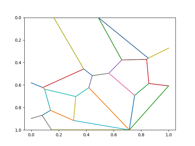
.. we can draw diagrams like..
basePoints = ({"x": 0.9676, "y": 0.4927}, {"x": 0.2163, "y": 0.7649}, {"x": 0.936, "y": 0.7093}, {"x": 0.206, "y": 0.4837}, {"x": 0.2662, "y": 0.5927}, {"x": 0.4211, "y": 0.7802}, {"x": 0.5706, "y": 0.663}, {"x": 0.5134, "y": 0.3368}, {"x": 0.7245, "y": 0.2413}, {"x": 0.0938, "y": 0.9428}, {"x": 0.79, "y": 0.1978}, {"x": 0.9625, "y": 0.7223}, {"x": 0.0454, "y": 0.804}, {"x": 0.7317, "y": 0.5099}, {"x": 0.1314, "y": 0.9227})
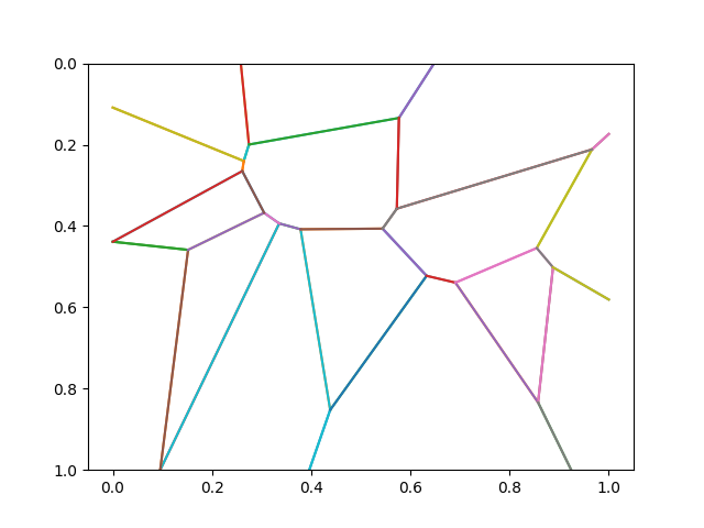
basePoints = ({"x": 0.3386, "y": 0.609}, {"x": 0.9819, "y": 0.4941}, {"x": 0.4702, "y": 0.5913}, {"x": 0.7416, "y": 0.3839}, {"x": 0.6513, "y": 0.698}, {"x": 0.8471, "y": 0.5873}, {"x": 0.4398, "y": 0.0989}, {"x": 0.0949, "y": 0.1276}, {"x": 0.6836, "y": 0.2273}, {"x": 0.186, "y": 0.5486}, {"x": 0.0724, "y": 0.5129}, {"x": 0.912, "y": 0.5932}, {"x": 0.4667, "y": 0.2232}, {"x": 0.0723, "y": 0.173}, {"x": 0.0892, "y": 0.3857})
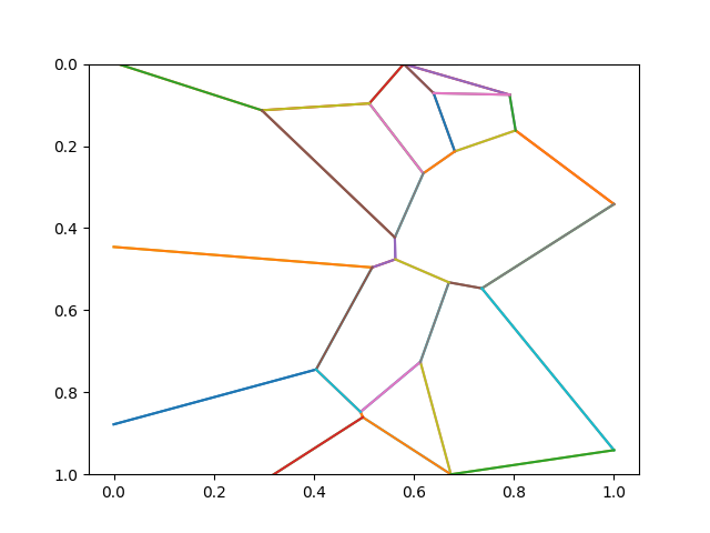
basePoints = ({"x": 0.4655, "y": 0.0055}, {"x": 0.6653, "y": 0.7868}, {"x": 0.3889, "y": 0.8753}, {"x": 0.6838, "y": 0.0881}, {"x": 0.5915, "y": 0.8032}, {"x": 0.7723, "y": 0.2991}, {"x": 0.6114, "y": 0.1098}, {"x": 0.4801, "y": 0.1928}, {"x": 0.8984, "y": 0.0585}, {"x": 0.6846, "y": 0.0564}, {"x": 0.3141, "y": 0.6487}, {"x": 0.3471, "y": 0.307}, {"x": 0.9848, "y": 0.5728}, {"x": 0.4576, "y": 0.9632}, {"x": 0.5361, "y": 0.7488})
Release history Release notifications | RSS feed


Download files
Download the file for your platform. If you're not sure which to choose, learn more about installing packages.
Source Distribution
Built Distribution
Filter files by name, interpreter, ABI, and platform.
If you're not sure about the file name format, learn more about wheel file names.
Copy a direct link to the current filters
File details
Details for the file voronout-0.0.3.tar.gz.
File metadata
- Download URL: voronout-0.0.3.tar.gz
- Upload date:
- Size: 186.9 kB
- Tags: Source
- Uploaded using Trusted Publishing? No
- Uploaded via: twine/6.2.0 CPython/3.14.0
File hashes
| Algorithm | Hash digest | |
|---|---|---|
| SHA256 |
c3b167a2db8f493c474c5df1e0aeb6b3f4d3306de356bd0b9c1cce2586914dee
|
|
| MD5 |
ac545dfc96ed09cf4baf5d7a58f2d825
|
|
| BLAKE2b-256 |
f8e2a1905290dd2d0c2df23cf39b4cc9813f9178498de361a99d4cccd96faae3
|
File details
Details for the file voronout-0.0.3-py3-none-any.whl.
File metadata
- Download URL: voronout-0.0.3-py3-none-any.whl
- Upload date:
- Size: 21.6 kB
- Tags: Python 3
- Uploaded using Trusted Publishing? No
- Uploaded via: twine/6.2.0 CPython/3.14.0
File hashes
| Algorithm | Hash digest | |
|---|---|---|
| SHA256 |
74baf3032ae7893408959641f33ce7b896d8eb7b6551854278ba33ab8c94340e
|
|
| MD5 |
e6afdd88bd1de9135c37ba7d2fdd9015
|
|
| BLAKE2b-256 |
59f2dc00f83dc7cb837cc7bfbf9a77ee0e1e69a76b2cdd071e8014fb62f11376
|


