
Wicksell-py
A Python class for computing Wicksell's transforms of continuous distributions.
Purpose
Consider a medium consisting in a large number of spheres whose radii follow a Probability Density Function (PDF) f. If sections of the medium are made at random lattitudes, the radius of apparent disks (denoted r below) would follow the PDF [1]:
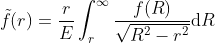
where E is the mean value of f. The previous formula is refered to as the Wicksell's equation.
The aim of this project is to provide a robust and convinient way to compute the statistics of apparents disks (related to values of r). It is based on histogram decomposition of f, as detailed in [2].
Installation
pip install Wicksell
Basic use
In your Python script, import the class constructor for WicksellTransform:
from Wicksell.transform import WicksellTransform
and create an instance of that class, passing the underlying distribution (that used for computing the Wicksell transform).
wt = WicksellTransform(distro)
In the example above, distro must be a continuous distribution, as defined in the scipy's stats module. Finally, use this instance as a usual scipy's distribution. Then all the parameters given to the wt function are actually passed-by and applied to the base-distribution (distro).
Example
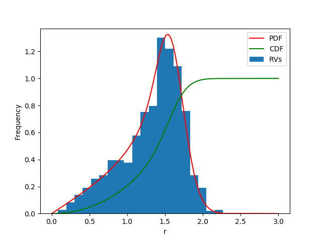
In the following, the lognormal distribion is considered.
import scipy.stats as stats
import numpy as np
from  Wicksell.transform import WicksellTransform

wlognorm = WicksellTransform(stats.lognorm)
s = 0.1                 # Shape parameter for lognormal
mu = 0.5
scale = np.exp(mu)  # loc parameter of underlying distribution
Compute the transformed PDF/CDF
x = np.linspace(0, 3, 1000)
pdf = wlognorm.pdf(x, s, scale=scale)
cdf = wlognorm.cdf(x, s, scale=scale)
Generate random variables
data = wlognorm.rvs(s, scale=scale, size=1000, random_state=0)
The random state is fixed here for reproductibility.
Plot results
from matplotlib import pyplot as plt

fig, ax1 = plt.subplots()
ax1.hist(data, bins=20, density=True, label='RVs')
ax1.set_ylim(bottom=0.0)
ax1.plot(x, pdf, 'r', label='PDF')
ax1.plot(x, cdf, 'g', label='CDF')
ax1.set_ylim(bottom=0.0)
ax1.legend()
ax1.set_xlabel('r')
ax1.set_ylabel('Frequency')
plt.show()
Fit the empirical data
Empirical data can be used to fit the distribution in odrer to get the optimal distribution parameters:
theta = wlognorm.fit(data, floc=0.0)
Here, the fit is made assuming that the location parameter is 0. The fit method is a build-in method provided in all rv_continuous distributions. See the related documentation for details.
The example below roughly leads to:
(0.10258798884347263, 0.0, 1.649539304907202)
It appears that the first parameter is close to s (0.1) whereas the scale (3rd one) corresponds to µ=ln(1.654)=0.5005 (instead of 0.5).
Perform a goodness of fit test
The transformed CDF can be used to perform the Kolmogorov-Smirnov test. For instance, the parameters evaluated by fitting lead to:
stats.kstest(data, wlognorm.cdf, theta)

KstestResult(statistic=0.020989374537414673, pvalue=0.7704283648898784)
:warning: Caveat :warning:
Using the histogram decomposition instead of computing the improper integral considerably speeds up the computation of the PDF/CDF. Still, it can be time consuming. Thus the fit method can be slow. Indeed, the example above takes about 100 seconds to complete on an Intel i9 @ 2.30 GHz.
Cite this work
If you use this tool in your research, please cite reference [2].
Community guidelines
Feel free to modify and contribute to this software in any manner, as long as your edit complies with the MIT licence. If you have troubles or want to report a bug, please use the issue tracker.
References
[1] Wicksell, S. D. (1925). The corpuscle problem: A mathematical study of a biometric problem. Biometrika, 17(1/2):84–99, DOI: 10.2307/2332027
[2] Depriester, D. and Kubler, R. (2021). Grain size estimation in polycrystals: solving the corpuscle problem using Maximum Likelihood Estimation. Journal of Structural Geology, 151:104418, ISSN 0191-8141, DOI: 10.1016/j.jsg.2021.104418
1 maintainer

Metadata
1 maintainer
Release files for Wicksell 2.1.0
For a detailed explanation of source distributions (sdists) and built distributions (wheels), please see the package formats documentation.
Source distribution (sdist)
| File | Size | Uploaded | |
|---|---|---|---|
| Wicksell-2.1.0.tar.gz | 7.8 kB | Details |
Built distribution (wheel)
| File | Interpreter | ABI | Platform | Reset |
|---|---|---|---|---|
| Wicksell-2.1.0-py3-none-any.whl | Python 3 | none | any | Details |
Total release size: 15.8 kB
Release files / Wicksell-2.1.0.tar.gz
| Download URL | Wicksell-2.1.0.tar.gz |
|---|---|
| Size | 7.8 kB |
| Tags | Source |
|
SHA-256 checksum How to use checksums |
d57839d8cfdb5f9a225ac55fa81b134c1a1f208582628a97c97d7592cfc5bc3e
|
|
BLAKE2b-256 checksum How to use checksums |
214ca771412e9d61b17ca01ab6ee6436f19dbb6d11cb87eba40fdc2afc213fc2
|
| Upload date | |
|
Uploaded using Trusted Publishing? What is trusted publishing? |
No |
| Uploaded via |
twine/4.0.1 CPython/3.9.15
|
Release files / Wicksell-2.1.0-py3-none-any.whl
| Download URL | Wicksell-2.1.0-py3-none-any.whl |
|---|---|
| Size | 7.9 kB |
| Tags | Python 3 |
|
SHA-256 checksum How to use checksums |
a4ca3957ab4d525ec0d75ca3d8c80d7e0d97528760fb99426e01e4f422c35572
|
|
BLAKE2b-256 checksum How to use checksums |
75bdaf322801c719543c5c6f77343ea133b8e4ab92c5e39eea70d5235e03a069
|
| Upload date | |
|
Uploaded using Trusted Publishing? What is trusted publishing? |
No |
| Uploaded via |
twine/4.0.1 CPython/3.9.15
|














