A python package to process Direct Numerical Simulations

Project description


A Python package to process Direct Numerical Simulations of reacting and non-reacting flows.
Purpose of the project
The project aims to help make large DNS (Direct Numerical Simulations) datasets more accessible to everyone, both to those who come from the field of Combustion and Fluid Dynamics, and who come from other fields. Processing DNS data can be challenging in several ways. This package offers:
- Field3D: An object that automatically reads formatted data aligned with Blastnet [1, 2], an open source scientific repository.
- Scalar3D: An object that efficiently manages pointers to local files, preventing memory overload.
- Plotting utilities: Generate visualizations with just one line of code, simplifying the validation process.
Functionalities
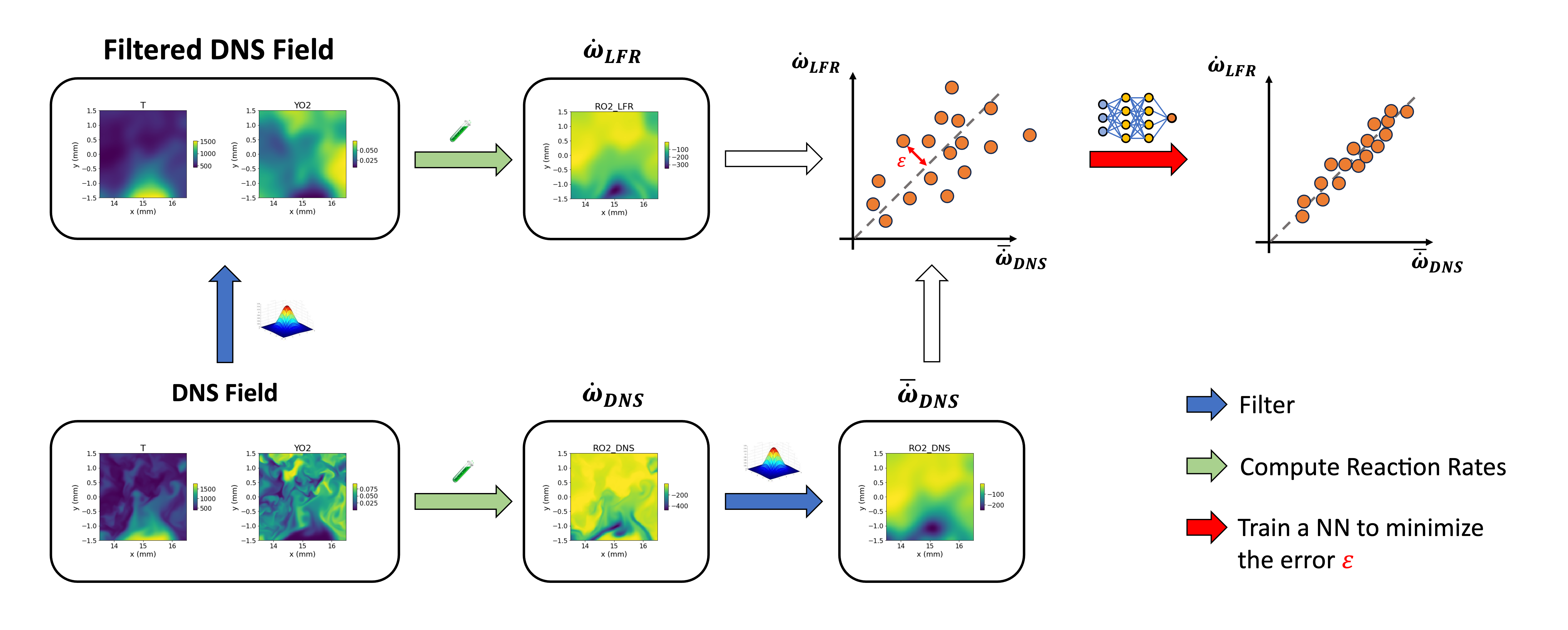
This library simplifies the standard workflow commonly used for a priori validation with DNS data. A priori validation is typically applied to assess turbulence and combustion models. More recently, this approach has been extended to train and evaluate machine learning models, which are increasingly utilized in the fluid dynamics community to enhance the accuracy of source term modeling.
The following figure displays the typical set of operations that using aPriori can be performed with a few lines of code:
Installation
Run the following command to install:
pip install aPrioriDNS
This will automatically install or update the following dependencies if necessary:
- numpy>=1.18.0,
- scipy>=1.12.0,
- matplotlib>=3.2.0,
- cantera>=3.0.0,
- tabulate>=0.9.0,
- requests>=2.32.0.
Documentation
The complete software documentation is available at:
https://apriori.gitbook.io/apriori-documentation-1
How to cite
This open-source software is distributed under the MIT license. If you use it in your work, please cite it as:
Lorenzo Piu. ‘aprioridns: V1.1.8’. Zenodo, 19 September 2024. https://doi.org/10.5281/zenodo.13793623.
Quickstart
The following code can be used to test the library once installed. A detailed explanation of the workflow presented is available here.
"""
Created on Fri May 24 14:50:44 2024

@author: lorenzo piu
"""

import aPrioriDNS as ap

# Download the dataset
ap.download()

# Initialize 3D DNS field
field_DNS = ap.Field3D('Lifted_H2_subdomain')

#----------------------------Visualize the dataset-----------------------------

# Plot Temperature on the xy midplane (transposed as yx plane)
field_DNS.plot_z_midplane('T',                 # plots the Temperature
                          levels=[1400, 2000], # isocontours at 1400 and 2000
                          vmin=1400,           # minimum temperature to plot
                          title='T [K]',       # figure title
                          linewidth=2,         # isocontour lines thickness
                          transpose=True,      # inverts x and y axes
                          x_name='y [mm]',     # x axis label
                          y_name='x [mm]')     # y axis label
# Plot Temperature on the xz midplane (transposed as zx plane)
field_DNS.plot_y_midplane('T',
                          levels=[1400, 2000],
                          vmin=1400,
                          title='T [K]',
                          linewidth=2,
                          transpose=True,
                          x_name='z [mm]',
                          y_name='x [mm]')
# Plot Temperature on the yz midplane
field_DNS.plot_x_midplane('T', levels=[1400, 2000], vmin=1400,
                          title='T [K]', linewidth=2)
# Plot OH mass fraction on the transposed xy midplane
field_DNS.plot_z_midplane('YOH', title=r'$Y_{OH}$', colormap='inferno',
                          transpose=True, x_name='z [mm]', y_name='x [mm]')

#--------------------------Compute DNS reaction rates--------------------------
field_DNS.compute_reaction_rates()

# Plot reaction rates
field_DNS.plot_z_midplane('RH2O_DNS',
                          title=r'$\dot{\omega}_{H2O}$ $[kg/m^3/s]$',
                          colormap='inferno',
                          transpose=True, x_name='z [mm]', y_name='x [mm]')
field_DNS.plot_z_midplane('ROH_DNS',
                          title=r'$\dot{\omega}_{OH}$ $[kg/m^3/s]$',
                          colormap='inferno',
                          transpose=True, x_name='z [mm]', y_name='x [mm]')

# compute kinetic energy
field_DNS.compute_kinetic_energy()

# Compute mixture fraction
field_DNS.ox = 'O2'     # Defines the species to consider as oxydizer
field_DNS.fuel = 'H2'   # Defines the species to consider as fuel
Y_ox_2=0.233  # Oxygen mass fraction in the oxydizer stream (air)
Y_f_1=0.65*2/(0.65*2+0.35*28) # Hydrogen mass fraction in the fuel stream
# (the fuel stream is composed by X_H2=0.65 and X_N2=0.35)

field_DNS.compute_mixture_fraction(Y_ox_2=Y_ox_2, Y_f_1=Y_f_1, s=2)

# Scatter plot variables as functions of the mixture fraction Z
field_DNS.scatter_Z('T', # the variable to plot on the y axis
                    c=field_DNS.YOH.value, # set color of the points
                    y_name='T [K]',
                    cbar_title=r'$Y_{OH}$'
                    )

field_DNS.scatter_Z('ROH_DNS',
                    c=field_DNS.HRR_DNS.value,
                    y_name=r'$\dot{\omega}_{OH}$ $[kg/m^3/s]$',
                    cbar_title=r'$\dot{Q}_{DNS}$'
                    )

#-------------------------------Filter DNS field-------------------------------
# perform favre filtering (high density gradients)
# the output of the function is a string with the new folder's name, f_string
f_string = field_DNS.filter_favre(filter_size=16, # filter amplitude
                                        filter_type='Gauss') # 'Gauss' or 'Box'

# The string with the folder's name is now used to initialize the filered field
field_filtered = ap.Field3D(f_string)

# Visualize the effect of filtering on the Heat Release Rate
field_DNS.plot_z_midplane('HRR_DNS',
                          title=r'$\dot{Q}_{DNS}$',
                          colormap='inferno',
                          vmax=8*1e9,
                          transpose=True, x_name='z [mm]', y_name='x [mm]')

field_filtered.plot_z_midplane('HRR_DNS',
                          title=r'$\overline{\dot{Q}_{DNS}}$',
                          colormap='inferno',
                          vmax=8*1e9,
                          transpose=True, x_name='z [mm]', y_name='x [mm]')

#-------------------------Compute reaction rates (LFR)-------------------------
# Computing reaction rates directly from the filtered field (LFR approximation)
field_filtered.compute_reaction_rates()

# Compare visually the results
field_filtered.plot_z_midplane('RH2_DNS',
                          title=r'$\overline{\dot{\omega}}_{H2,DNS}$',
                          vmax=-20,
                          vmin=field_filtered.RH2_LFR.z_midplane.min(),
                          levels=[-300, -50, -20],
                          labels=True,
                          colormap='inferno',
                          transpose=True, x_name='z [mm]', y_name='x [mm]')

# Compare visually the results in the z midplane
field_filtered.plot_z_midplane('RH2_LFR',
                          title=r'$\overline{\dot{\omega}}_{H2,LFR}$',
                          vmax=-20,
                          vmin=field_filtered.RH2_LFR.z_midplane.min(),
                          levels=[-300, -50, -20],
                          labels=True,
                          colormap='inferno',
                          transpose=True, x_name='z [mm]', y_name='x [mm]')

# Compare the heat release rate results with a parity plot
f = ap.parity_plot(field_filtered.HRR_DNS.value,  # x
                   field_filtered.HRR_LFR.value,  # y
                   density=True,                  # KDE coloured
                   x_name=r'$\overline{\dot{\omega}}_{H2,DNS}$',
                   y_name=r'$\overline{\dot{\omega}}_{H2,LFR}$'
                   )
Bibliography
[1] W. T. Chung, B. Akoush, P. Sharma, A. Tamkin, K. S. Jung, J. H. Chen, J. Guo, D. Brouzet, M. Talei, B. Savard, A.Y. Poludnenko & M. Ihme. Turbulence in Focus: Benchmarking Scaling Behavior of 3D Volumetric Super-Resolution with BLASTNet 2.0 Data. Advances in Neural Information Processing Systems (2023) 36.
[2] W. T. Chung, M. Ihme, K. S. Jung, J. H. Chen, J. Guo, D. Brouzet, M. Talei, B. Jiang, B. Savard, A. Y. Poludnenko, B. Akoush, P. Sharma & A. Tamkin. BLASTNet Simulation Dataset (Version 2.0), 2023. https://blastnet.github.io/.
Release history Release notifications | RSS feed


Download files
Download the file for your platform. If you're not sure which to choose, learn more about installing packages.
Source Distribution
Built Distribution
Filter files by name, interpreter, ABI, and platform.
If you're not sure about the file name format, learn more about wheel file names.
Copy a direct link to the current filters
File details
Details for the file aprioridns-1.1.10.tar.gz.
File metadata
- Download URL: aprioridns-1.1.10.tar.gz
- Upload date:
- Size: 2.0 MB
- Tags: Source
- Uploaded using Trusted Publishing? No
- Uploaded via: twine/5.0.0 CPython/3.11.6
File hashes
| Algorithm | Hash digest | |
|---|---|---|
| SHA256 |
90bc75cf2fd0ebc3c926071853dacf250a9ad44fa5576ec782a8be5fbd338fc5
|
|
| MD5 |
428dcf9128da22c8106e6d3ca585bf12
|
|
| BLAKE2b-256 |
e510987aff83ed9e6aa83995ad5cb3a99fc558164fe912d4c526be39e7b7999e
|
File details
Details for the file aprioridns-1.1.10-py3-none-any.whl.
File metadata
- Download URL: aprioridns-1.1.10-py3-none-any.whl
- Upload date:
- Size: 57.9 kB
- Tags: Python 3
- Uploaded using Trusted Publishing? No
- Uploaded via: twine/5.0.0 CPython/3.11.6
File hashes
| Algorithm | Hash digest | |
|---|---|---|
| SHA256 |
383ae70e42c776d2cfbf383ffcb7bc261fabc0a22098210ba8bf8264aa6ba1f8
|
|
| MD5 |
086780817e2292c90bc66e2cb801b14a
|
|
| BLAKE2b-256 |
053d2344297326c6cf70f6033b33fc13ea6e207b6ab00fd829f70e173604322f
|


