Transforms PMV-based into adaptive setpoint temperature EnergyPlus building energy models

Project description


ACCIM stands for Adaptive-Comfort-Control-Implemented Model.
In research terms, this is a proposal for a paradigm shift, from using fixed PMV-based to adaptive setpoint temperatures, based on adaptive thermal comfort algorithms and it has been widely studied and published on scientific research journals (for more information, refer to https://orcid.org/0000-0002-3080-0821).
In terms of code, this is a python package that transforms fixed setpoint temperature building energy models into adaptive setpoint temperature energy models by adding the Adaptive Comfort Control Implementation Script (ACCIS). This package has been developed to be used in EnergyPlus building energy performance simulations.
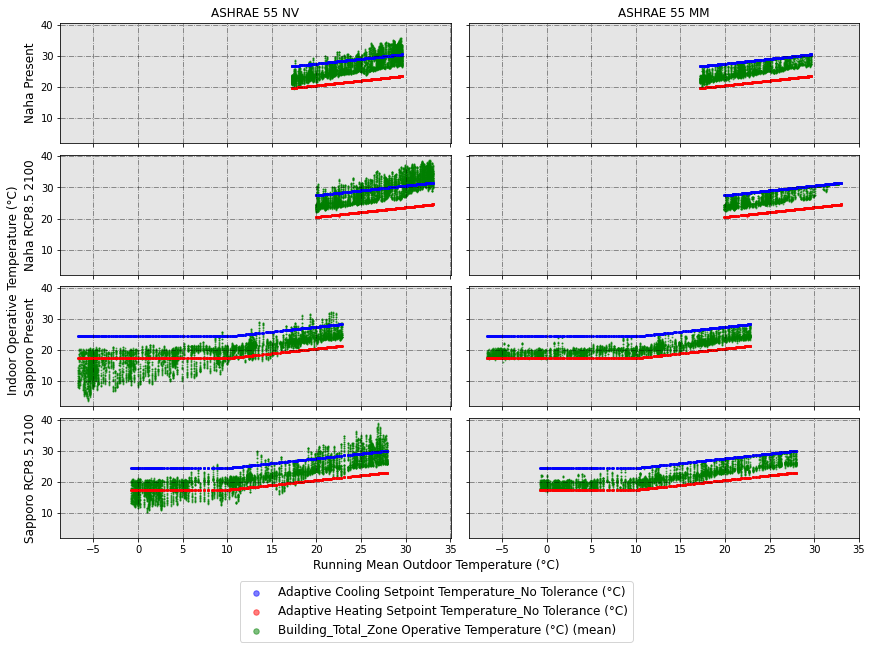
The figure below clearly explains the aim of adaptive setpoint temperatures: introducing hourly temperature values into the adaptive comfort zone. On the left column, you can see the simulation results of a naturally ventilated building, while on the right column, the same building in mixed-mode operation with adaptive setpoint temperatures.
1. Citation
If you use this package, please cite us:
[1] D. Sánchez-García, David Bienvenido-Huertas, Carlos Rubio-Bellido, Computational approach to extend the air-conditioning usage to adaptive comfort: Adaptive-Comfort-Control-Implementation Script, Automation in Construction 131 (2021) 103900. doi:10.1016/j.autcon.2021.103900. https://doi.org/10.1016/j.autcon.2021.103900
[2] Daniel Sánchez-García, Jorge Martínez-Crespo, Ulpiano Ruiz-Rivas Hernando, Carmen Alonso, A detailed view of the Adaptive-Comfort-Control-Implementation Script (ACCIS): The capabilities of the automation system for adaptive setpoint temperatures in building energy models, Energy and Buildings 288 (2023) 113019. doi:10.1016/j.enbuild.2023.113019. https://doi.org/10.1016/j.enbuild.2023.113019
[3] Daniel Sánchez-García, David Bienvenido-Huertas, William O’Brien, accim: a Python library for adaptive setpoint temperatures in building performance simulations, Journal of Building Performance Simulation (2025) 1–13. doi:10.1080/19401493.2025.2472305. https://doi.org/10.1080/19401493.2025.2472305
[3] Daniel Sánchez-García, David Bienvenido-Huertas, Alberto Cerezo-Narváez, Mc. Delgado Guerrero, José Sánchez Ramos, A methodological framework and computational tool for adaptive predicted mean vote setpoints in EnergyPlus building simulations, Journal of Building Engineering. 119 (2026) 115273. doi:10.1016/j.jobe.2026.115273. https://doi.org/10.1016/j.jobe.2026.115273
2. How to use
2.0 Requirements
To use accim, the following must be installed:
- Python 3.9 or newer
- EnergyPlus (any version between 9.1 and 25.1 those included)
2.1 Installation
First of all, you need to install the package:
pip install accim
2.2 Usage
2.2.1 Transforming PMV-based into adaptive setpoint temperatures
This is a very brief explanation of the usage. Therefore, if you don't get the results you expected or get some error, I would recommend reading the 'Detailed use' section at the documentation in the link https://accim.readthedocs.io/en/master/
accim will take as input IDF files those located at the same path as the script. You only need to run the following code:
2.2.1.1 Short version
from accim.sim import accis
accis.addAccis()
Once you run this code, you will be asked to enter some information at the terminal or python console to generate the output IDF files.
2.2.1.2 Longer version
from accim.sim import accis
accis.addAccis(
    ScriptType=str, # ScriptType: 'vrf_mm', 'vrf_ac', 'ex_mm', 'ex_ac'. For instance: ScriptType='vrf_ac',
    SupplyAirTempInputMethod=str, # SupplyAirTempInputMethod: 'supply air temperature', 'temperature difference'. For instance: SupplyAirTempInputMethod='supply air temperature',
    Output_keep_existing=bool, # Output_keep_existing: True or False. For instance: Output_keep_existing=False,
    Output_type=str, # Output_type: 'simplified', 'standard', 'detailed' or 'custom'. For instance: Output_type='standard',
    Output_freqs=list, # Output_freqs: ['timestep', 'hourly', 'daily', 'monthly', 'runperiod']. For instance: Output_freqs=['hourly', 'runperiod'],
    Output_gen_dataframe=bool, # Output_keep_existing: True or False. For instance: Output_keep_existing=False,
    Output_take_dataframe=pandas Dataframe,
    EnergyPlus_version=str, # EnergyPlus_version: '9.1', '9.2', '9.3', '9.4', '9.5', '9.6', '22.1', '22.2', '23.1', '23.2', '24.1', '24.2', '25.1' or 'auto'. For instance: EnergyPlus_version='25.1',
    TempCtrl=str, # TempCtrl: 'temperature' or 'temp', or 'pmv'. For instance: TempCtrl='temp',
    ComfStand=list, # it is the Comfort Standard. Can be any integer from 0 to 22. For instance: ComfStand=[0, 1, 2, 3],
    CAT=list, # it is the Category. Can be 1, 2, 3, 80, 85 or 90. For instance: CAT=[3, 80],
    ComfMod=list, # it is Comfort Mode. Can be 0, 1, 2 or 3. For instance: ComfMod=[0, 3],
    SetpointAcc=float, # it is the accuracy of the setpoint temperatures
    CoolSeasonStart=dd/mm date in string format or integer to represent the day of the year, # it is the start date for the cooling season
    CoolSeasonEnd=dd/mm date in string format or integer to represent the day of the year, # it is the end date for the cooling season
    HVACmode=list, # it is the HVAC mode. 0 for Full AC, 1 for NV and 2 for MM. For instance: HVACmode=[0, 2],
    VentCtrl=list, # it is the Ventilation Control. Can be 0 or 1. For instance: VentCtrl=[0, 1],
    MaxTempDiffVOF=float, # When the difference of operative and outdoor temperature exceeds MaxTempDiffVOF, windows will be opened the fraction of MultiplierVOF. For instance: MaxTempDiffVOF=20,
    MinTempDiffVOF=float, # When the difference of operative and outdoor temperature is smaller than MinTempDiffVOF, windows will be fully opened. Between min and max, windows will be linearly opened. For instance: MinTempDiffVOF=1,
    MultiplierVOF=float, # Fraction of window to be opened when temperature difference exceeds MaxTempDiffVOF. For instance: Multiplier=0.2,
    VSToffset=list, # it is the offset for the ventilation setpoint. Can be any number, float or int. For instance: VSToffset=[-1.5, -1, 0, 1, 1.5],
    MinOToffset=list, # it is the offset for the minimum outdoor temperature to ventilate. Can be any positive number, float or int. For instance: MinOToffset=[0.5, 1, 2],
    MaxWindSpeed=list, # it is the maximum wind speed allowed for ventilation. Can be any positive number, float or int. For instance: MinOToffset=[2.5, 5, 10],
    ASTtol_start=float, # it is the start of the tolerance sequence. For instance: ASTtol_start=0,
    ASTtol_end_input=float, # it is the end of the tolerance sequence. For instance: ASTtol_start=2,
    ASTtol_steps=float, # these are the steps of the tolerance sequence. For instance: ASTtol_steps=0.25,
    NameSuffix=str # NameSuffix: some text you might want to add at the end of the output IDF file name. For instance: NameSuffix='whatever',
    verboseMode=bool # verboseMode: True to print all process in screen, False to not to print it. Default is True. For instance: verboseMode=True,
    confirmGen=bool # True to confirm automatically the generation of IDFs; if False, you'll be asked to confirm in command prompt. Default is False. For instance: confirmGen=False,
)
You can see a Jupyter Notebook in the link below:
https://github.com/dsanchez-garcia/accim/blob/master/accim/sample_files/jupyter_notebooks/addAccis/using_addAccis.ipynb
You can also execute it at your computer. You just need to find the folder containing the .ipynb and all other files at the accim package folder within your site_packages path, in
accim/sample_files/jupyter_notebooks/addAccis
The path should be something like this, with your username instead of YOUR_USERNAME:
C:\Users\YOUR_USERNAME\AppData\Local\Programs\Python\Python39\Lib\site-packages\accim\sample_files\jupyter_notebooks\addAccis
Then, you just need to copy the folder to a different path (i.e. Desktop), open a cmd dialog pointing at it, and run "jupyter notebook". After that, an internet browser will pop up, and you will be able to open the .ipynb file.
2.2.2 Renaming epw files for later data analysis
You can see a Jupyter Notebook in the link below:
https://github.com/dsanchez-garcia/accim/blob/master/accim/sample_files/jupyter_notebooks/rename_epw_files/using_rename_epw_files.ipynb
You can also execute it at your computer. You just need to find the folder containing the .ipynb and all other files at the accim package folder within your site_packages path, in
accim/sample_files/jupyter_notebooks/rename_epw_files
The path should be something like this, with your username instead of YOUR_USERNAME:
C:\Users\YOUR_USERNAME\AppData\Local\Programs\Python\Python39\Lib\site-packages\accim\sample_files\jupyter_notebooks\rename_epw_files
Then, you just need to copy the folder to a different path (i.e. Desktop), open a cmd dialog pointing at it, and run "jupyter notebook". After that, an internet browser will pop up, and you will be able to open the .ipynb file.
2.2.3 Running simulations
You can see a Jupyter Notebook in the link below:
https://github.com/dsanchez-garcia/accim/blob/master/accim/sample_files/jupyter_notebooks/runEp/using_runEp.ipynb
You can also execute it at your computer. You just need to find the folder containing the .ipynb and all other files at the accim package folder within your site_packages path, in
accim/sample_files/jupyter_notebooks/runEp
The path should be something like this, with your username instead of YOUR_USERNAME:
C:\Users\YOUR_USERNAME\AppData\Local\Programs\Python\Python39\Lib\site-packages\accim\sample_files\jupyter_notebooks\runEp
Then, you just need to copy the folder to a different path (i.e. Desktop), open a cmd dialog pointing at it, and run "jupyter notebook". After that, an internet browser will pop up, and you will be able to open the .ipynb file.
2.2.4 Functions and methods for data analysis; making figures and tables
You can see a Jupyter Notebook in the link below:
https://github.com/dsanchez-garcia/accim/blob/master/accim/sample_files/jupyter_notebooks/Table/using_Table.ipynb
You can also execute it at your computer. You just need to find the folder containing the .ipynb and all other files at the accim package folder within your site_packages path, in
accim/sample_files/jupyter_notebooks/Table
The path should be something like this, with your username instead of YOUR_USERNAME:
C:\Users\YOUR_USERNAME\AppData\Local\Programs\Python\Python39\Lib\site-packages\accim\sample_files\jupyter_notebooks\Table
Then, you just need to copy the folder to a different path (i.e. Desktop), open a cmd dialog pointing at it, and run "jupyter notebook". After that, an internet browser will pop up, and you will be able to open the .ipynb file.
2.2.5 Full example: from preparation of the input IDFs and EPWs, to simulation and data analysis and visualization
You can see a Jupyter Notebook in the link below:
https://github.com/dsanchez-garcia/accim/blob/master/accim/sample_files/jupyter_notebooks/full_example_IBPSA/full_example_IBPSA.ipynb
This Notebook was used in the IBPSA webinar (although for accim version 0.7.1), which you can watch at the following YouTube link: https://www.youtube.com/watch?v=PQ34Pl7t4HA&t=3393s
You can also execute it at your computer. You just need to find the folder containing the .ipynb and all other files at the accim package folder within your site_packages path, in
accim/sample_files/jupyter_notebooks/full_example_IBPSA
The path should be something like this, with your username instead of YOUR_USERNAME:
C:\Users\YOUR_USERNAME\AppData\Local\Programs\Python\Python39\Lib\site-packages\accim\sample_files\jupyter_notebooks\full_example_IBPSA
Then, you just need to copy the folder to a different path (i.e. Desktop), open a cmd dialog pointing at it, and run "jupyter notebook". After that, an internet browser will pop up, and you will be able to open the .ipynb file.
2.2.6 Using apmv_setpoints
You can see a Jupyter Notebook in the link below:
https://github.com/dsanchez-garcia/accim/blob/master/accim/sample_files/jupyter_notebooks/example_apmv_setpoints_paper/using_apmv_setpoints.ipynb
You can also execute it at your computer. You just need to find the folder containing the .ipynb and all other files at the accim package folder within your site_packages path, in
accim/sample_files/jupyter_notebooks/example_apmv_setpoints_paper
The path should be something like this, with your username instead of YOUR_USERNAME:
C:\Users\YOUR_USERNAME\AppData\Local\Programs\Python\Python39\Lib\site-packages\accim\sample_files\jupyter_notebooks\example_apmv_setpoints_paper
Then, you just need to copy the folder to a different path (i.e. Desktop), open a cmd dialog pointing at it, and run "jupyter notebook". After that, an internet browser will pop up, and you will be able to open the .ipynb file.
You can apply aPMV setpoints to a building using the following function:
from accim.sim import apmv_setpoints
apmv_setpoints.apply_apmv_setpoints(
    building=IDF_object, # building: the comprehensive eppy or besos IDF object
    outputs_freq=list, # outputs_freq: ['timestep', 'hourly', 'daily', 'monthly', 'runperiod']. For instance: Output_freqs=['hourly', 'runperiod'],
    other_PMV_related_outputs=bool, # other_PMV_related_outputs: True to include other PMV related outputs (e.g. Fanger PMV, PPD, etc). Default is True.
    adap_coeff_cooling=float or dict, # adap_coeff_cooling: Adaptive coefficient (lambda) for cooling. Can be a single float (applied globally) or a dict {TargetName: Value}. Default is 0.293.
    adap_coeff_heating=float or dict, # adap_coeff_heating: Adaptive coefficient (lambda) for heating. Float or Dict {TargetName: Value}. Default is -0.293.
    pmv_cooling_sp=float or dict, # pmv_cooling_sp: Target PMV setpoint for cooling (e.g., 0.5). Float or Dict. Default is 0.5.
    pmv_heating_sp=float or dict, # pmv_heating_sp: Target PMV setpoint for heating (e.g., -0.5). Float or Dict. Default is -0.5.
    tolerance_cooling_sp_cooling_season=float or dict, # tolerance_cooling_sp_cooling_season: Tolerance to widen the cooling setpoint band during cooling season. Float or Dict. Default is -0.1.
    tolerance_cooling_sp_heating_season=float or dict, # tolerance_cooling_sp_heating_season: Tolerance to widen the cooling setpoint band during heating season. Float or Dict. Default is -0.1.
    tolerance_heating_sp_cooling_season=float or dict, # tolerance_heating_sp_cooling_season: Tolerance to widen the heating setpoint band during cooling season. Float or Dict. Default is 0.1.
    tolerance_heating_sp_heating_season=float or dict, # tolerance_heating_sp_heating_season: Tolerance to widen the heating setpoint band during heating season. Float or Dict. Default is 0.1.
    cooling_season_start=int or str, # cooling_season_start: Start day of the cooling season. Can be an integer (Day of Year) or string ('dd/mm'). Default is 120 (May 1st approx).
    cooling_season_end=int or str, # cooling_season_end: End day of the cooling season. Can be an integer (Day of Year) or string ('dd/mm'). Default is 210 (July 29th approx).
    dflt_for_adap_coeff_cooling=float, # dflt_for_adap_coeff_cooling: Default value for cooling adaptive coefficient if key is missing in dict input. Default is 0.4.
    dflt_for_adap_coeff_heating=float, # dflt_for_adap_coeff_heating: Default value for heating adaptive coefficient if key is missing in dict input. Default is -0.4.
    dflt_for_pmv_cooling_sp=float, # dflt_for_pmv_cooling_sp: Default value for cooling PMV setpoint if key is missing in dict input. Default is 0.5.
    dflt_for_pmv_heating_sp=float, # dflt_for_pmv_heating_sp: Default value for heating PMV setpoint if key is missing in dict input. Default is -0.5.
    dflt_for_tolerance_cooling_sp_cooling_season=float, # dflt_for_tolerance_cooling_sp_cooling_season: Default tolerance value if key is missing. Default is -0.1.
    dflt_for_tolerance_cooling_sp_heating_season=float, # dflt_for_tolerance_cooling_sp_heating_season: Default tolerance value if key is missing. Default is -0.1.
    dflt_for_tolerance_heating_sp_cooling_season=float, # dflt_for_tolerance_heating_sp_cooling_season: Default tolerance value if key is missing. Default is 0.1.
    dflt_for_tolerance_heating_sp_heating_season=float, # dflt_for_tolerance_heating_sp_heating_season: Default tolerance value if key is missing. Default is 0.1.
    verbose_mode=bool # verbose_mode: True to print detailed progress messages (added objects) and warnings to the console. Default is True.
)
3. Documentation
Detailed documentation, including the explanation of the different arguments, is at: https://accim.readthedocs.io/en/master/
4. Project Funding
This software has been funded by the following projects, which include the following research articles as research outputs:
- "NAIPE - Nuevo Análisis Integral de la Pobreza Energética en Andalucía. Predicción, evaluación y adaptación al cambio climático de hogares vulnerables desde una perspectiva económica, ambiental y social" (US- 125546) funded by the European Regional Development Fund (ERDF) and by the “Consejería de Economía y Conocimiento de la Junta de Andalucía (Spain)”. Research outputs: [1, 2, 3, 4, 5]
- "RIPEBA - Red Iberoamericana de Pobreza Energética y Bienestar Ambiental" (Thematic Network 722RT0135) financed by the call for Thematic Networks of the CYTED Program for 2021. Research outputs: [7, 8, 9, 10, 11, 12, 13]
- "IBERESE - Red Iberoamericana de Eficiencia y Salubridad en Edificios" (Thematic Network 723RT0151) financed by the call for Thematic Networks of the CYTED Program for 2022. Research outputs: [10, 12, 13, 14]
- "EPIU - Energy Poverty Intelligence Unit" (UIA04-212) by the Urban Innovative Actions initiative (European Commission). Research outputs: [6, 9, 10, 12]
- "+ENERPOT - Positive Energy Buildings Potential for Climate Change Adaptation and Energy Poverty Mitigation" (PID2021-122437OA-I00) by the Spanish Ministry of Science, Innovation and Universities. Research outputs: [7, 8, 9, 10, 11, 12]
- "ImplicAdapt - Implicaciones en la mitigación del cambio climático y de la pobreza energética mediante nuevo modelo de confort adaptativo para viviendas sociales" (US.22-02) by the Andalusian Ministry of Development, Articulation of the Territory and Housing. Research outputs: [7, 8, 9, 11, 12]
- "CONSTANCY - Resilient urbanisation methodologies and natural conditioning using imaginative nature-based solutions and cultural heritage to recover the street life" (Grant Agreement PID2020-118972RB-I00) by the Spanish Ministry of Science, Innovation and Universities. Research outputs: [14]
- "COSMIC - Combined AI and Data Solutions for Large Scale Resource Optimization with Green Deal Impact" (Grant Agreement GA-101189676) by the European Commission. Research outputs: [14, 15]
- Vitality – Project Code ECS00000041, CUP I33C22001330007 - funded under the National Recovery and Resilience Plan (NRRP), Mission 4 Component 2 Investment 1.5 - 'Creation and strengthening of innovation ecosystems,' construction of 'territorial leaders in R&D' – Innovation Ecosystems - Project 'Innovation, digitalization and sustainability for the diffused economy in Central Italy – VITALITY' Call for tender No. 3277 of 30/12/2021, and Concession Decree No. 0001057.23-06-2022 of Italian Ministry of University funded by the European Union – NextGenerationEU. Research outputs: [14]
- LIFE BUILD-OSS: OSS Training Programa Leading Energy Efficiency for BUILDing” (LIFE24-CET-BUILD-OSS), by the European Commission. Research outputs: [15]
References:
- [1] D. Bienvenido-Huertas, D. Sánchez-García, C. Rubio-Bellido, Analysing natural ventilation to reduce the cooling energy consumption and the fuel poverty of social dwellings in coastal zones, Appl. Energy. 279 (2020) 115845. doi:10.1016/j.apenergy.2020.115845. https://www.doi.org/10.1016/j.apenergy.2020.115845
- [2] D. Bienvenido-Huertas, D. Sánchez-García, C. Rubio-Bellido, J.A. Pulido-Arcas, Applying the mixed-mode with an adaptive approach to reduce the energy poverty in social dwellings: The case of Spain, Energy. 237 (2021) 121636. doi:10.1016/j.energy.2021.121636. https://www.doi.org/10.1016/j.energy.2021.121636
- [3] D. Bienvenido-Huertas, D. Sánchez-García, C. Rubio-Bellido, Adaptive setpoint temperatures to reduce the risk of energy poverty? A local case study in Seville, Energy Build. 231 (2021) 110571. doi:10.1016/j.enbuild.2020.110571. https://www.doi.org/10.1016/j.enbuild.2020.110571
- [4] D. Bienvenido-Huertas, D. Sánchez-García, C. Rubio-Bellido, D. Marín-García, Potential of applying adaptive strategies in buildings to reduce the severity of fuel poverty according to the climate zone and climate change: The case of Andalusia, Sustain. Cities Soc. 73 (2021) 103088. doi:10.1016/j.scs.2021.103088. https://www.doi.org/10.1016/j.scs.2021.103088
- [5] D. Bienvenido-Huertas, D. Sánchez-García, C. Rubio-Bellido, Influence of the RCP scenarios on the effectiveness of adaptive strategies in buildings around the world, Build. Environ. 208 (2022) 108631. doi:10.1016/j.buildenv.2021.108631. https://www.doi.org/10.1016/j.buildenv.2021.108631
- [6] D. Sánchez-García, J. Martínez-Crespo, U.R.-R. Hernando, C. Alonso, A detailed view of the Adaptive-Comfort-Control-Implementation Script (ACCIS): The capabilities of the automation system for adaptive setpoint temperatures in building energy models, Energy Build. 288 (2023) 113019. doi:10.1016/j.enbuild.2023.113019. https://www.doi.org/10.1016/j.enbuild.2023.113019
- [7] D. Bienvenido-Huertas, D. Sánchez-García, D. Marín-García, C. Rubio-Bellido, Analysing energy poverty in warm climate zones in Spain through artificial intelligence, J. Build. Eng. 68 (2023) 106116. doi:10.1016/j.jobe.2023.106116. https://www.doi.org/10.1016/j.jobe.2023.106116
- [8] D. Bienvenido-Huertas, D. Sánchez-García, D. Marín-García, C. Rubio-Bellido, Is the analysis scale crucial to assess energy poverty? analysis of yearly and monthly assessments using the 2 M indicator in the south of Spain, Energy Build. 285 (2023) 112889. doi:10.1016/j.enbuild.2023.112889. https://www.doi.org/10.1016/j.enbuild.2023.112889
- [9] D. Sánchez-García, D. Bienvenido-Huertas, J.A. Pulido-Arcas, C. Rubio-Bellido, Extending the use of adaptive thermal comfort to air-conditioning: The case study of a local Japanese comfort model in present and future scenarios, Energy Build. 285 (2023) 112901. doi:10.1016/j.enbuild.2023.112901. https://www.doi.org/10.1016/j.enbuild.2023.112901
- [10] D. Sánchez-García, D. Bienvenido-Huertas, J. Martínez-Crespo, R. de Dear, Using setpoint temperatures based on adaptive thermal comfort models: The case of an Australian model considering climate change, Build. Environ. 258 (2024) 111647. doi:10.1016/j.buildenv.2024.111647. https://www.doi.org/10.1016/j.buildenv.2024.111647
- [11] D. Bienvenido-Huertas, D. Sánchez-García, C. Rubio-Bellido, D. Marín-García, Holistic analysis to reduce energy poverty in social dwellings in southern Spain considering envelope, systems, operational pattern, and income levels, Energy. 288 (2024) 129796. doi:10.1016/j.energy.2023.129796. https://www.doi.org/10.1016/j.energy.2023.129796
- [12] D. Sánchez-García, D. Bienvenido-Huertas, C. Rubio-Bellido, R.F. Rupp, Assessing the energy saving potential of using adaptive setpoint temperatures: The case study of a regional adaptive comfort model for Brazil in both the present and the future, Build. Simul. 17 (2024) 459–482. doi:10.1007/s12273-023-1084-3. https://www.doi.org/10.1007/s12273-023-1084-3
- [13] D. Sánchez-García, D. Bienvenido-Huertas, W. O’Brien, accim: a Python library for adaptive setpoint temperatures in building performance simulations, J. Build. Perform. Simul. (2025) 1–13. doi:10.1080/19401493.2025.2472305. https://www.doi.org/10.1080/19401493.2025.2472305
- [14] D. Sánchez-García, D. Bienvenido-Huertas, J. Kim, A.L. Pisello, Exploring the energy implications of human thermal adaptation to hot temperatures in present and future scenarios: a parametric simulation study, Energy. 325 (2025) 136029. doi:10.1016/j.energy.2025.136029. https://www.doi.org/10.1016/j.energy.2025.136029
- [15] D. Sánchez-García, D. Bienvenido-Huertas, A. Cerezo-Narváez, Mc. Delgado Guerrero, J. Sánchez Ramos, A methodological framework and computational tool for adaptive predicted mean vote setpoints in EnergyPlus building simulations, Journal of Building Engineering. 119 (2026) 115273. https://doi.org/10.1016/j.jobe.2026.115273.
5. Credits
It wouldn't have been possible to develop this python package without eppy and besos, so thank you for such an awesome work.
Release history Release notifications | RSS feed


Download files
Download the file for your platform. If you're not sure which to choose, learn more about installing packages.
Source Distribution
Built Distribution
Filter files by name, interpreter, ABI, and platform.
If you're not sure about the file name format, learn more about wheel file names.
Copy a direct link to the current filters
File details
Details for the file accim-0.7.7.tar.gz.
File metadata
- Download URL: accim-0.7.7.tar.gz
- Upload date:
- Size: 38.0 MB
- Tags: Source
- Uploaded using Trusted Publishing? No
- Uploaded via: twine/6.2.0 CPython/3.9.13
File hashes
| Algorithm | Hash digest | |
|---|---|---|
| SHA256 |
11535e177b014dc13a8a669fdb8b55eeed06321a5091e2bf9b297f05e0b46233
|
|
| MD5 |
7826ae555ca47ae978268444c73a8971
|
|
| BLAKE2b-256 |
db811440ae7af72632534e14d6e7dcc6461e35139adf51c1ebad89053c96cacf
|
File details
Details for the file accim-0.7.7-py3-none-any.whl.
File metadata
- Download URL: accim-0.7.7-py3-none-any.whl
- Upload date:
- Size: 38.5 MB
- Tags: Python 3
- Uploaded using Trusted Publishing? No
- Uploaded via: twine/6.2.0 CPython/3.9.13
File hashes
| Algorithm | Hash digest | |
|---|---|---|
| SHA256 |
4eccde85d6ecad9f776f69c7fbe70bf25eae37ad226aaaaf3d185383bcb6da34
|
|
| MD5 |
48cad0e933ab21938c2453a739e5e2cf
|
|
| BLAKE2b-256 |
bc709256be225192e34a1e449533ede6a71e464faa939d4a70f96ca0e6fb8583
|


