
adaptive_cut




Hierarchical clustering usually ends with one horizontal cut of the dendrogram, so every cluster is taken at the same height. When clusters have different densities or scales, no single height fits all of them.
The adaptive cut cuts each branch of the dendrogram at its own height. Among
all such multi-level cuts, it returns the one that maximises an objective
summed over clusters. adaptive_cut does this for any scipy linkage matrix:
point clouds, networks, or anything else you can build a dendrogram for.
The method is described in L. Boucherie, Y.-Y. Ahn, S. Lehmann, Adaptive cut reveals multiscale complexity in networks, PNAS Nexus (2026), doi:10.1093/pnasnexus/pgag344.
Install
pip install adaptive_cut              # numpy + scipy only
pip install "adaptive_cut[numba]"     # compiled sampler, 20-50x faster
pip install "adaptive_cut[all]"       # numba + networkx
From a clone of the repository: pip install -e ".[all,test]", then pytest.
The examples and the tutorial notebook also need
pip install "adaptive_cut[examples]" (matplotlib and scikit-learn).
Example: clusters at different scales
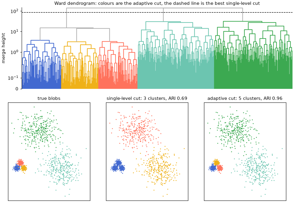
The figure above comes from
examples/points.py.
The data have three tight blobs next to two wide ones, clustered by Ward
linkage. Each cluster is scored by the BIC of one Gaussian fitted to it, so the
sum over a cut is the BIC of a Gaussian mixture with one component per cluster.
from scipy.cluster.hierarchy import linkage
import adaptive_cut as ac
from points import blobs, gaussian_scores     # examples/points.py

X, y = blobs(seed=0)
Z = linkage(X, "ward")
scores = gaussian_scores(X, Z)                # one score per dendrogram node
level = ac.best_level_cut(Z, scores)          # 3 clusters, ARI 0.69
best = ac.optimal_cut(Z, scores)              # 5 clusters, ARI 0.96
A height that separates the three tight blobs also cuts the wide blobs into pieces, so the best single-level cut (dashed line) merges the tight blobs instead. The adaptive cut (colours) takes the tight blobs low in the tree and the wide blobs high.
How it works
Cuts and scores. Nodes follow scipy's numbering for a linkage matrix Z
with n leaves:
- leaves are
0 .. n-1; - row
iofZcreates noden + i; - the root is
2n - 2.
A cut is a set of nodes whose subtrees partition the leaves. You give one score
per node, an array scores of length 2n - 1 where scores[v] is the value of
the cluster made of the leaves under v. The objective of a cut is
scores[cut.nodes].sum(), and it is maximised. To minimise a cost, negate it.
Exact optimum. Because the objective is a sum over clusters, its maximum
over all cuts follows from one bottom-up pass over the tree,
best(v) = max(scores[v], best(left) + best(right)). optimal_cut does this
in O(n) time. On ties it keeps the larger cluster.
Single-level cut. best_level_cut returns the best horizontal cut, the
usual baseline. It tries every distinct merge height and applies tied merges
together, as fcluster(Z, h, "distance") does.
Sampler. adaptive_cut is the Markov chain of the paper. It samples cuts
from exp(f(cut) / T) with a reversible-jump Metropolis-Hastings chain:
- Pick: choose a current cluster uniformly at random.
- Direction: leaves move up and the root moves down; any other cluster moves up or down with probability 1/2.
- Up: merge the cluster with its sibling into their parent. If the sibling is itself split, all clusters below it are merged as well.
- Down: replace the cluster by a sub-cut
sof its subtree, drawn with probability proportional to2^-|s|. At least one child stays whole, so the move can be reversed in one step. - Accept the move with the Metropolis-Hastings ratio, which includes the exact proposal probabilities.
- Anneal: the temperature is
Tup to stepk_sa(default2/3 n_steps), thenT / ln(k - k_sa + 2).
The chain starts from the best single-level cut. It returns the best cut
visited (res.best), the last state (res.final) and a trace of the objective
(res.trace). Use it to explore near-optimal cuts. To get the maximum, use
optimal_cut: the chain can stall where improving the cut first requires a
worse one. On the blobs above, the chain at T="auto" stays at the
single-level cut.
- Temperature:
Tis in units of the objective.T="auto"sets it to 0.1 times the median absolute change of the objective over the single merges of the dendrogram. - Steps:
n_stepsdefaults tomax(10_000, 10 n). Use 10^4 or more for a few thousand leaves, and 10^5 to 10^6 for larger trees.
Your own clustering and objective
Any scipy linkage matrix and any per-cluster score work.
node_scores(Z, func) calls func(leaf_ids) on every node and returns the
scores array.
from scipy.cluster.hierarchy import linkage
import adaptive_cut as ac

Z = linkage(X, "average")                        # any scipy dendrogram
scores = ac.node_scores(Z, my_cluster_score)     # my_cluster_score(leaf_ids) -> float
level = ac.best_level_cut(Z, scores)             # best horizontal cut
best = ac.optimal_cut(Z, scores)                 # adaptive cut, exact
res = ac.adaptive_cut(Z, scores, T="auto", rng=0)  # adaptive cut, sampled

best.value, best.n_clusters, best.labels
node_scores calls func once per node, so its cost grows with the sum of all
subtree sizes. For large trees, compute the scores bottom-up, as
gaussian_scores in examples/points.py does from per-node counts, sums and
sums of squares.
examples/any_dendrogram.py
clusters the nodes of a network by average linkage on shortest-path distances,
with modularity as the objective.
Networks: link communities
link_communities runs the whole pipeline for a network. It clusters the
edges by the Jaccard similarity of their endpoints' neighbourhoods (single
linkage), scores every cluster by partition density, and returns the best
single-level cut and the adaptive cut.
import numpy as np
import adaptive_cut as ac

edges = np.loadtxt("network.txt", dtype=int)   # one "u v" pair per line
r = ac.link_communities(edges, rng=0)

r.level_cut.value       # partition density D of the best single-level cut
r.partition_density     # D of the adaptive cut
r.cut.labels            # community of every edge (edge i is r.edges[i])
r.communities()         # node labels of every (overlapping) link community
r.memberships()         # sparse (nodes x communities) fraction of each node's edges
r.Z, r.scores           # the edge dendrogram and its scores, for optimal_cut etc.
graph can be an edge array of any sortable labels, a networkx.Graph, or a
symmetric scipy.sparse adjacency matrix. For weighted networks pass
weights= with an edge array, or weighted=True with a graph or matrix.
Here T="auto" is clip(0.1/M * f_D, 1e-8, 1e-3) for M edges, with
f_D = 0.3 when the single-level D > 0.7, 0.01 when D < 0.01, else 1.
examples/sbm.py
builds two stochastic block models with five blocks each:
- Varying density: block densities run from 1 down to 0.1, and sparser blocks are larger.
- Balanced: five equal blocks with density 0.9 inside and 0.1 between.
import numpy as np
import adaptive_cut as ac

def sbm(sizes, P, seed):
    rng = np.random.default_rng(seed)
    block = np.repeat(np.arange(len(sizes)), sizes)
    i, j = np.triu_indices(len(block), 1)
    keep = rng.random(i.size) < np.asarray(P)[block[i], block[j]]
    return np.column_stack([i[keep], j[keep]])

p = np.linspace(1, 0.1, 5)
P = np.diag(p)
for c in range(4):
    P[c, c + 1] = P[c + 1, c] = p[c + 1] ** 2
varying = sbm((20 / np.sqrt(p)).astype(int), P, seed=0)
balanced = sbm([40] * 5, 0.1 + 0.8 * np.eye(5), seed=0)

for name, edges in [("varying density", varying), ("balanced", balanced)]:
    r = ac.link_communities(edges, n_steps=50_000, rng=0)
    print(f"{name:>16}: M={len(r.edges):5d}  B={r.balancedness:.2f}  "
          f"D single-level={r.level_cut.value:.3f} ({r.level_cut.n_clusters} communities)  "
          f"D adaptive={r.partition_density:.3f} ({r.cut.n_clusters} communities)")
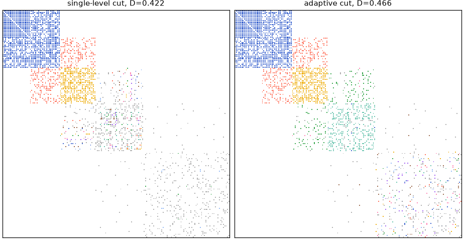
 varying density: M= 1550  B=0.26  D single-level=0.422 (386 communities)  D adaptive=0.466 (152 communities)
        balanced: M= 5105  B=0.66  D single-level=0.618 (16 communities)  D adaptive=0.619 (14 communities)
In the varying-density network, dense blocks merge low in the edge dendrogram and sparse blocks merge high, so no single height suits every block. The adaptive cut raises the partition density from 0.422 to 0.466. In the balanced network all blocks merge at similar heights, and the single-level cut is already as good as the adaptive one.
Each edge of the varying-density network, coloured by its link community (communities of one or two edges in grey). The single-level cut that suits the dense blocks leaves the fourth block in fragments; the adaptive cut groups it.
Classic datasets
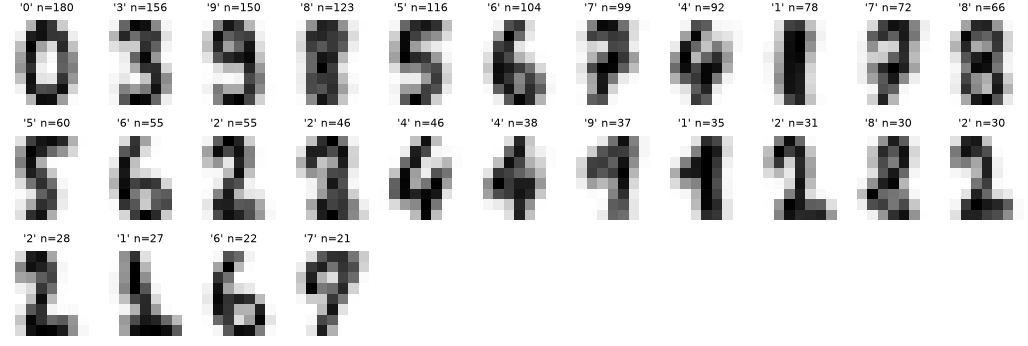
The Gaussian score with Ward linkage, on iris and wine (standardised) and digits (reduced to 10 PCA dimensions). The adaptive cut raises the objective, but the agreement with the true classes (ARI) changes little, in both directions. The objective is not the class labels. For digits the change depends on the preprocessing: from -0.02 to +0.11 ARI with 5 to 30 PCA dimensions.
| Dataset | Points | B | Single-level cut | Adaptive cut |
|---|---|---|---|---|
| iris | 150 | 0.94 | 4 clusters, ARI 0.59 | 5 clusters, ARI 0.57 |
| wine | 178 | 0.94 | 3 clusters, ARI 0.79 | 3 clusters, ARI 0.79 |
| digits | 1,797 | 0.97 | 29 clusters, ARI 0.47 | 26 clusters, ARI 0.58 |
Mean image of each digits cluster of the adaptive cut, with its most common digit and its size:
Balancedness
balancedness(Z) describes how evenly a dendrogram splits its leaves, level by
level. Every distinct merge height of Z defines a level: the partition
obtained by applying all merges up to that height, with tied merges applied
together. Each level splits the n leaves into k clusters, and is compared
with two reference splits:
His the Shannon entropy (base 2) of the cluster sizes;H_maxis the entropy of the most even split ofnintokclusters;H_minis the entropy of the most skewed split (k - 1singletons).
Then
B = mean over levels of (H - H_min) / (H_max - H_min)
The mean runs over all levels where H_max > H_min, that is 2 <= k <= n - 2.
B = 1when every level is as even as possible.B = 0for a caterpillar dendrogram, where each merge adds a single leaf.Bisnanwhen no level is informative.
balancedness(Z, return_levels=True) also returns the per-level values.
Performance and reproducibility
- Exact optimum:
optimal_cutis one pass over then - 1merges. - Sampler: each step costs O(1) plus the size of the proposed move. The state lives in flat integer arrays, and the proposal tables are precomputed once per tree.
- Engines: with numba installed the compiled sampler is used
(
engine="auto"). The pure-Python engine runs the same code. Both engines give identical results for the samerng, which CI checks on Linux, macOS and Windows. - Link clustering:
- The similarities come from one sparse matrix product.
- The dendrogram comes from scipy's minimum spanning tree over the edge
pairs. A dense
scipy.cluster.hierarchy.linkagecall would need memory quadratic in the number of edges. - Memory grows with the number of edge pairs that share a node,
sum_v deg(v)(deg(v)-1)/2, so hubs dominate.
Measured on one core (numpy 2.4, scipy 1.17, numba 0.68). "Dendrogram" is
link_communities(..., adaptive=False): similarities, linkage, scores,
balancedness and the single-level cut.
| Network | Edges | Edge pairs | Dendrogram | Sampler, numba | Sampler, Python |
|---|---|---|---|---|---|
| Zachary karate club | 78 | 528 | < 0.01 s | 0.13 µs/step | 4 µs/step |
| euroroad | 1,305 | 2.7k | 0.02 s | 0.24 µs/step | 9 µs/step |
| bible_nouns | 9,059 | 368k | 0.26 s | 5.3 µs/step | 240 µs/step |
| us_roads-VT | 104,644 | 157k | 0.85 s | 6.6 µs/step | 130 µs/step |
| marvel_universe | 95,445 | 12.8M | 9.3 s | 24 µs/step | 540 µs/step |
The cost of a step grows with the number of clusters a move touches, so networks with many small clusters under large ones are slower per step.
API
| Function | Purpose |
|---|---|
optimal_cut(Z, scores) |
Adaptive cut, exact; returns Cut |
adaptive_cut(Z, scores, T, ...) |
Adaptive cut by MCMC; returns AdaptiveCutResult |
best_level_cut(Z, scores) |
Best single-level cut; returns Cut |
node_scores(Z, func) |
Per-node scores from a per-cluster function |
link_communities(graph, ...) |
Link clustering of a network; returns LinkCommunities |
partition_density_scores(Z, edges) |
Per-node partition density of an edge dendrogram |
balancedness(Z, return_levels=False) |
Balancedness of a dendrogram |
Citation
@article{boucherie2026adaptive,
  title   = {Adaptive cut reveals multiscale complexity in networks},
  author  = {Boucherie, Louis and Ahn, Yong-Yeol and Lehmann, Sune},
  journal = {PNAS Nexus},
  year    = {2026},
  doi     = {10.1093/pnasnexus/pgag344}
}
License
MIT
1 maintainer

Metadata
1 maintainer
Release files for adaptive-cut 0.1.0
For a detailed explanation of source distributions (sdists) and built distributions (wheels), please see the package formats documentation.
Source distribution (sdist)
| File | Size | Uploaded | Provenance | Actions |
|---|---|---|---|---|
| adaptive_cut-0.1.0.tar.gz | 353.3 kB | With provenance | Details for adaptive_cut-0.1.0.tar.gz |
Built distribution (wheel)
| File | Interpreter | ABI | Platform | Actions Reset |
|---|---|---|---|---|
| adaptive_cut-0.1.0-py3-none-any.whl | Python 3 | none | any | Details for adaptive_cut-0.1.0-py3-none-any.whl |
Total release size: 380.7 kB
Release files / adaptive_cut-0.1.0.tar.gz
| Download URL | adaptive_cut-0.1.0.tar.gz |
|---|---|
| Size | 353.3 kB |
| Tags | Source |
|
SHA-256 checksum How to use checksums |
b73a388fc1b4691dc192b01f5eac99a29250025dbb533750b46e3d3a1ac05410
|
|
BLAKE2b-256 checksum How to use checksums |
1a31f47a8745e4025457e198ecaff2a3e73d0d38620853b7b8bebfeb8e6a366d
|
| Upload date | |
|
Uploaded using Trusted Publishing? What is trusted publishing? |
Yes |
| Uploaded via |
twine/7.0.0 CPython/3.13.16
|
Provenance
Provenance describes where a file came from. On PyPI, provenance is shared via attestations, which provide a verifiable record of the build or publishing details. View details, limitations and caveats.


PyPI Publish Attestation
PyPI verified that this artifact, at this checksum, originated from the publisher listed below.
Signed by GitHub Actions, verified by PyPI on Oct 22, 2026.
Transparency logRelease files / adaptive_cut-0.1.0-py3-none-any.whl
| Download URL | adaptive_cut-0.1.0-py3-none-any.whl |
|---|---|
| Size | 27.4 kB |
| Tags | Python 3 |
|
SHA-256 checksum How to use checksums |
bd05d636041d076b8c726a899bb08d905bcbb8fd919f2098d4b1b65413fdbe47
|
|
BLAKE2b-256 checksum How to use checksums |
a149a6cfe9ec303118a569cd7d47fd14a68a65733a89fbc4ea181fe3b3318292
|
| Upload date | |
|
Uploaded using Trusted Publishing? What is trusted publishing? |
Yes |
| Uploaded via |
twine/7.0.0 CPython/3.13.16
|
Provenance
Provenance describes where a file came from. On PyPI, provenance is shared via attestations, which provide a verifiable record of the build or publishing details. View details, limitations and caveats.
PyPI Publish Attestation
PyPI verified that this artifact, at this checksum, originated from the publisher listed below.
Signed by GitHub Actions, verified by PyPI on Oct 22, 2026.
Transparency logSecurity for adaptive-cut 0.1.0
Provenance
Provenance describes where a file came from. On PyPI, provenance is shared via attestations, which provide a verifiable record of the build or publishing details. View details, limitations and caveats.
Full provenance
All 2 files in this release have been uploaded with provenance metadata.
Attestation for adaptive_cut-0.1.0.tar.gz
PyPI Publish Attestation
PyPI verified that this artifact, at this checksum, originated from the publisher listed below.
Signed by GitHub Actions, verified by PyPI on Oct 22, 2026.
Transparency logA note on package security
PyPI is a repository for distributing packages, not a service for auditing them. While third-party security researchers and our staff do their best to detect and remove malicious packages, PyPI cannot guarantee the quality, security or suitability of any given package.
To learn more about protecting yourself from malicious actors, visit our package security documentation.














