Because using satellite data should not be rocket science.

Project description
AgriGEE.lite
AgriGEE.lite is an Earth Engine wrapper that allows easy download of Analysis Ready Multimodal Data (ARD), focused on downloading time series of agricultural and native vegetation data.
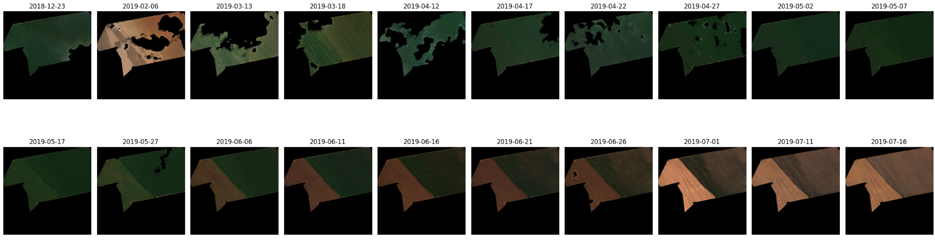
For example, to download and view a time series of cloud-free Sentinel 2 imagery cropped to a specific field and date range, only a few lines of code are required. Here’s an example:
import agrigee_lite as agl
import ee

ee.Initialize()

gdf = gpd.read_parquet("data/sample.parquet")
row = gdf.iloc[0]

satellite = agl.sat.Sentinel2(bands=["red", "green", "blue"])
agl.vis.images(row.geometry, row.start_date, row.end_date, satellite)
Through this example, it is already possible to understand the basic functioning of the lib. The entire lib was designed to be used in conjunction with GeoPandas, and a basic knowledge of it is necessary.
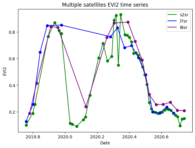
You can also download aggregations, such as spatial median aggregations of indices. Here's an example with median from multiple satellites:
For more examples, see the examples folder.
Finally, the library features multithreaded downloading, which allows downloading on average 16-22 time series per second (assuming 1-year series, cloud-free for Sentinel 2 BOA).
The lib has 3 types of elements, which are divided into modules:
-
agl.sat = Data sources, usually coming from satellites/sensors. When defining a sensor, it is possible to choose which bands you want to view/download, or whether you want to use atmospheric corrections or not. By default, all bands are downloaded, and all atmospheric corrections and harmonizations are used.
-
agl.vis = Module that allows you to view data, either through time series or images.
-
agl.get = Module that allows you to download data on a large scale.
Available data sources (satellites, sensors, models and so on)
| Name | Bands | Start Date | End Date | Regionality | Pixel Size | Revisit Time | Variations |
|---|---|---|---|---|---|---|---|
| Sentinel 2 | Blue, Green, Red, Re1, Re2, Re3, Nir, Re4, Swir1, Swir2 | 2016-01-01 | (still operational) | Worldwide | 10 -- 60 | 5 days | BOA, TOA |
| Landsat 5 | Blue, Green, Red, Nir, Swir1, Swir2 | 1984-03-01 | 2013-05-05 | Worldwide* | 15 -- 30 | 16 days | BOA, TOA; Tier 1 and Tier 2; |
| Landsat 7 | Blue, Green, Red, Nir, Swir1, Swir2, Pan | 1999-04-15 | 2022-04-06 | Worldwide* | 15 -- 30 | 16 days | BOA, TOA; Tier 1 and Tier 2; Pan-sharpened |
| Landsat 8 | Blue, Green, Red, Nir, Swir1, Swir2, Pan | 2013-04-11 | (still operational) | Worldwide | 15 -- 30 | 16 days | BOA, TOA; Tier 1 and Tier 2; Pan-sharpened |
| Landsat 9 | Blue, Green, Red, Nir, Swir1, Swir2, Pan | 2021-11-01 | (still operational) | Worldwide | 15 -- 30 | 16 days | BOA, TOA; Tier 1 and Tier 2; Pan-sharpened |
| MODIS Daily, 8 days | Red, Nir | 2000-02-18 | (still operational) | Worldwide | 15 -- 30 | daily/8 days | |
| Sentinel 1 | VV, VH - C Band | 2014-10-03 | (still operational) | Worldwide* | 10** | 5 days**** | GRD, ARD*** |
| JAXOS PalSAR 1/2 | HH, HV - L Band | 2014-08-04 | (still operational) | Worldwide | 25** | 15 days | GRD |
| Satellite Embeddings V1 | 64-dimensional embedding | 2017-01-01 | 2024-01-01 | Worldwide | 10 | 1 year | |
| Mapbiomas Brazil | 37 Land Usage Land Cover Classes | 1985-01-01 | 2024-12-31 | Brazil | 30 | 1 year | |
| ANADEM | Slope, Elevation, Aspect | (single image) | (single image) | South America | 30** | (single image) | |
| SoilGrids classes | WRB Soil Classes (30 categories) | (single image) | (single image) | Worldwide | 250 | (single image) |
Observations
- *Landsat 7 images began to have artifacts caused by a sensor problem from 2003-05-31.
- **Pixel size/spatial resolution for active sensors (or models that use active sensors) often lacks a clear value, as it depends on the angle of incidence. Here, the GEE value itself is explained, representing the highest resolution captured.
- ***Analysis Ready Data (ARD) is an advanced post-processing method applied to a SAR. However, it is quite costly, and its usefulness must be evaluated on a case-by-case basis.
- ****Sentinel 1 was a twin satellite, one of which went out of service due to a malfunction. Therefore, the revisit time varies greatly depending on the desired geolocation.
Available indices
| Index Name | Full Name | Required Bands | Sensor Type | Equation | Description |
|---|---|---|---|---|---|
| NDVI | Normalized Difference Vegetation Index | NIR, RED | Optical | $\frac{NIR - RED}{NIR + RED}$ | Vegetation greenness |
| GNDVI | Green Normalized Difference Vegetation Index | NIR, GREEN | Optical | $\frac{NIR - GREEN}{NIR + GREEN}$ | Vegetation health (chlorophyll) |
| NDWI | Normalized Difference Water Index | NIR, SWIR1 | Optical | $\frac{NIR - SWIR1}{NIR + SWIR1}$ | Water content |
| MNDWI | Modified Normalized Difference Water Index | GREEN, SWIR1 | Optical | $\frac{GREEN - SWIR1}{GREEN + SWIR1}$ | Water body detection |
| SAVI | Soil Adjusted Vegetation Index | NIR, RED | Optical | $\frac{(NIR - RED)}{(NIR + RED + 0.5)} \times 1.5$ | Vegetation, reduces soil effect |
| EVI | Enhanced Vegetation Index | NIR, RED, BLUE | Optical | $2.5 \times \frac{NIR - RED}{NIR + 6 \times RED - 7.5 \times BLUE + 1}$ | Vegetation, minimizes atmospheric effects |
| EVI2 | Two-band Enhanced Vegetation Index | NIR, RED | Optical | $2.5 \times \frac{NIR - RED}{NIR + 2.4 \times RED + 1}$ | Simplified EVI, no blue band |
| MSAVI | Modified Soil Adjusted Vegetation Index | NIR, RED | Optical | $\frac{2 \times NIR + 1 - \sqrt{(2 \times NIR + 1)^2 - 8 \times (NIR - RED)}}{2}$ | Vegetation in areas with bare soil |
| NDRE | Normalized Difference Red Edge Index | NIR, RE1 | Optical | $\frac{NIR - RE1}{NIR + RE1}$ | Chlorophyll content in leaves |
| MCARI | Modified Chlorophyll Absorption in Reflectance Index | NIR, RED, GREEN | Optical | $\left[(NIR - RED) - 0.2 \times (NIR - GREEN)\right] \times \frac{NIR}{RED}$ | Leaf chlorophyll content |
| GCI | Green Chlorophyll Index | NIR, GREEN | Optical | $\frac{NIR}{GREEN} - 1$ | Chlorophyll concentration |
| BSI | Bare Soil Index | BLUE, RED, NIR, SWIR1 | Optical | $\frac{(SWIR1 + RED) - (NIR + BLUE)}{(SWIR1 + RED) + (NIR + BLUE)}$ | Bare soil index |
| CI Red | Red Chlorophyll Index | NIR, RED | Optical | $\frac{NIR}{RED} - 1$ | Chlorophyll index (red) |
| CI Green | Green Chlorophyll Index | NIR, GREEN | Optical | $\frac{NIR}{GREEN} - 1$ | Chlorophyll index (green) |
| OSAVI | Optimized Soil Adjusted Vegetation Index | NIR, RED | Optical | $\frac{NIR - RED}{NIR + RED + 0.16}$ | Like SAVI, for low vegetation |
| ARVI | Atmospherically Resistant Vegetation Index | NIR, RED, BLUE | Optical | $\frac{NIR - (2 \times RED - BLUE)}{NIR + (2 \times RED - BLUE)}$ | Vegetation, reduces atmospheric effects |
| VHVV | VH/VV Ratio | VH, VV | Radar | $\frac{VH}{VV}$ | Vegetation structure (Sentinel-1) |
| HHHV | HH/HV Ratio | HH, HV | Radar | $\frac{HH - HV}{HH + HV}$ | Vegetation structure (PALSAR) |
| RVI | Radar Vegetation Index | HH, HV | Radar | $4 \times \frac{HV}{HH + HV}$ | Radar vegetation index (PALSAR) |
| RAVI | Radar Adapted Vegetation Index | VV, VH | Radar | $4 \times \frac{VH}{VV + VH}$ | Radar vegetation index (Sentinel-1) |
Avaiable reductors
| Name to Use | Full Name | Description |
|---|---|---|
| min | Minimum | Returns the smallest value in the set |
| max | Maximum | Returns the largest value in the set |
| mean | Mean | Returns the average of all values |
| median | Median | Returns the median (middle) value |
| kurt | Kurtosis | Returns the kurtosis (measure of "tailedness") |
| skew | Skewness | Returns the skewness (measure of asymmetry) |
| std | Standard Deviation | Returns the standard deviation |
| var | Variance | Returns the variance |
| mode | Mode | Returns the most frequent value |
| pXX | Percentile XX | Returns the XX-th percentile (e.g., p10 for 10th percentile). You can pass multiple, e.g., p10, p90. |
Motivations: what an average data scientist - me - thought when I started learning GEE
My journey with GEE started two and a half years ago. GEE is excellent, it allows you to use several different satellite data, but it is very complex to code. In addition to using A LOT of boilerplate code, the errors are extremely confusing, since the tool is executed server-side, most likely with a pure functional language (like Haskell). During my master's degree, I struggled a lot writing codes for GEE. Furthermore, harmonizing all satellites at the same time is difficult. Typically, each satellite has a different range of values and cloud masks. Tired of having to rewrite similar codes, I decided to create a lib with a simple goal: using satellite data should be as simple as reading a CSV in Pandas, and you shouldn't need to be a Remote Sensing expert to achieve it.
Objectives and target audience
The main objective of the lib is to be a simple, direct and high-performance way to download satellite data, both for academic and commercial use. Did you like it? Give it a star. Want to contribute? Open your Pull Request, I will be happy to include it.
Questions possibly asked
But isn't it just a case of using STAC? Why pay Google?
This is a tempting proposition, and it actually makes sense for large scale projects. However, processing satellite data locally can easily escalate to hell, especially for countries with huge agricultural areas like Australia, the United States or Brazil. So, you have to do the math to figure out whether it is cheaper or not to use GEE than to have your own processing infrastructure than STAC. However, GEE is completely free for students and non-commercial projects.
"Hello, I am a Remote Sensing expert, and I believe that the term satellite is not the most appropriate, radars do not have bands and.... "
Yes, I was told that. The use of the term "satellite" instead of sensor, data source or something else is intended to simplify things, even though it is not the most correct term. Note that even Mapbiomas, a WONDERFUL project that is made using models and AMAZING PEOPLE (❤️) is called a satellite, and is treated exactly the same as Sentinel 2 or any Landsat. The same goes for the idea of "bands" in a radar like Sentinel 1. The more standardized it is, the easier it is to keep the library code working. However, note that your help to the project is VERY WELCOME.
The library mascot is cute! Did you make it?
Absolutely not, I'm terrible at drawings and anything. I made it using GPT4, and all the rights belong to God knows who. The base art is from the Odd-Eyes Venom Dragon card from the Yu-Gi-Oh card game. The inspiration has nothing to do with venom, but rather because it is a plant dragon (agriculture), it is a fusion card (multimodal data) and it has odd-eyes (like satellites, seeing the world through different eyes). If you're a cartoonist and want to design a new mascot, I'd be more than happy to make it official.
Known Bugs
- QuadTree clustering functions produce absurd results when there are very uneven geographic density distributions, for example, thousands of points in one country and a few dozen in another. Some prior geospatial partitioning is recommended.
TO-DO
- Add Sentinel 2 as a satellite;
- Add Landsats 5, 7, 8, 9 as a satellite;
- Add Sentinel 1 GRD as a satellite;
- Add Mapbiomas Brazil as a satellite (data source);
- Add MODIS Terra/Acqua;
- Add Satellite Image Time Series Aggregations online download;
- Add Satellite Image Time Series Aggregations task download;
- Add Images online download/visualization with matplotlib;
- Add single/multiple SITS visualization
- Add smart_open[gcs] for autorecovery SITS from GCS;
- Add ALOS-2 PALSAR-2 radar;
- Add Images online visualization with plotly;
- Make cloud mask removable;
- Add all other Mapbiomas;
- Add Sentinel 1 ARD;
- Add Sentinel 3;
- Add jurassic Landsats (1-4);
- Add Landsat Pansharpening for image download;
Release history Release notifications | RSS feed


Download files
Download the file for your platform. If you're not sure which to choose, learn more about installing packages.
Source Distribution
Built Distribution
Filter files by name, interpreter, ABI, and platform.
If you're not sure about the file name format, learn more about wheel file names.
Copy a direct link to the current filters
File details
Details for the file agrigee_lite-2.0.6.tar.gz.
File metadata
- Download URL: agrigee_lite-2.0.6.tar.gz
- Upload date:
- Size: 54.1 kB
- Tags: Source
- Uploaded using Trusted Publishing? No
- Uploaded via: twine/6.2.0 CPython/3.11.10
File hashes
| Algorithm | Hash digest | |
|---|---|---|
| SHA256 |
8c9cb377a1f364dfe274e87b44d2b15319a80dfeeab1e6ebd655d69448ef7291
|
|
| MD5 |
0848b712e0acaa10a3b32f10c0aa1af7
|
|
| BLAKE2b-256 |
9df1f05b67d12f81a66166a22e93a59503589eb90852f0bfe8aaea43734e66f9
|
File details
Details for the file agrigee_lite-2.0.6-py3-none-any.whl.
File metadata
- Download URL: agrigee_lite-2.0.6-py3-none-any.whl
- Upload date:
- Size: 86.6 kB
- Tags: Python 3
- Uploaded using Trusted Publishing? No
- Uploaded via: twine/6.2.0 CPython/3.11.10
File hashes
| Algorithm | Hash digest | |
|---|---|---|
| SHA256 |
4a2b494ec35679232bb565d0c1193b038b7ab14e36f783bc2cc708ec16e3b8f2
|
|
| MD5 |
75831bbf1af26857bb1443f60b45b596
|
|
| BLAKE2b-256 |
0b8153154fb722a603750c80aecadf215d78944c20709e6b3fdfe963a1f720cd
|


