A Python package for stock portfolio analysis and optimization.

Project description
AnalyzerPortfolio
AnalyzerPortfolio is a Python package designed for comprehensive portfolio analysis, offering a powerful and user-friendly toolkit for investors, analysts, and researchers. Built primarily on yfinance, it allows users to retrieve financial data, construct portfolios, and evaluate their performance using industry-standard metrics such as beta, alpha, Sharpe ratio, Sortino ratio, Value-at-Risk (VaR), and more.
The package also features advanced visualization tools powered by plotly, enabling interactive and insightful graphical representations of portfolio performance. Additionally, AnalyzerPortfolio supports various portfolio optimization techniques, including minimum variance optimization, Sharpe ratio maximization, and information ratio optimization.
Furthermore, the package integrates AI-driven capabilities for real-time stock news monitoring and automated investment report generation, helping users stay informed and make data-driven decisions.
Installation
You can install AnalyzerPortfolio via pip:
pip install analyzerportfolio
Alternatively you can install AnalyzerPortfolio directly from GitHub using the following command:
pip install git+https://github.com/washednico/analyzerportfolio.git
Dependencies
AnalyzerPortfolio relies on the following Python libraries:
openai>=1.43.0– For AI-powered features (e.g., stock news monitoring, report generation)pandas>=1.5.1– For data manipulation and analysisyfinance>=0.2.32– For retrieving financial datanumpy==1.26.4– For numerical computationsplotly>=5.18.0– For interactive data visualizationarch>=7.0.0– For financial econometrics and risk modelingscipy==1.14.0– For mathematical and statistical computationsstatsmodels==0.14.1– For statistical modeling and hypothesis testingnbformat>=4.2.0– For working with Jupyter Notebook formats
To manually install the dependencies, run:
pip install openai pandas yfinance numpy plotly arch scipy statsmodels nbformat
Note that nbformat is required not directly for analyzerportfolio but indirectly for plotly, solving plotting issues.
Basic Usage
Below are examples demonstrating how to use AnalyzerPortfolio to:
- Calculate various portfolio metrics
- Generate graphical outputs
- Optimize a portfolio
- Analyze stock newss
Neverthless, users are highly encouraged to utilize the docstring help function (help(function_name)) to fully understand how each function works.
Scraping Financial Data
To retrieve market data using yfinance, you should use the download_data function. Below is an example of how to access its documentation:
print(ap.download_data.__doc__)
Download stock and market data, convert to base currency, and return the processed data.

Parameters:
- tickers (list): List of stock tickers.
- market_ticker (str): Market index ticker.
- start_date (str): Start date for historical data.
- end_date (str): End date for historical data.
- base_currency (str): The base currency for the portfolio (e.g., 'USD').
- risk_free (str): The risk free rate to use in the calculations written as ticker on fred (e.g., 'DTB3' for USD).
- use_cache (bool): Whether to use cache to retrieve data, if data is not cached it will be stored for future computations. Default is False.
- folder_path (str): Path to the folder where the cache will be stored. Default is None.

Returns:
pd.DataFrame: DataFrame containing the adjusted and converted prices for all tickers and the market index.
Examples: Scraping Financial Data
ticker = ['AAPL','MSFT','GOOGL','AMZN','TSLA','E']
investments = [100,200,300,300,200,500]
start_date = '2019-01-01'
end_date = '2024-08-28'
market_ticker = '^GSPC'
base_currency = 'EUR'
risk_free = "PCREDIT8"
rebalancing_period_days = 250
# Download historical data
data = ap.download_data(tickers=ticker, start_date=start_date, end_date=end_date, base_currency=base_currency,market_ticker=market_ticker, risk_free=risk_free)
Build portfolio object
Once market data are successfully scraped, the user should use create_portfolio to create a portfolio that is a requirement to perform any further computation.
print(ap.create_portfolio.__doc__)
Calculates returns and value amounts for specified stocks over a return period,
the portfolio without rebalancing, optionally the portfolio with auto-rebalancing,
and includes market index calculations.

Parameters:
- data: DataFrame with adjusted closing prices (index as dates, columns as tickers).
- tickers: List of stock tickers in the portfolio.
- investments: List or array of initial investments for each stock.
- market_ticker: String representing the market index ticker.
- name_portfolio: String representing the name of the portfolio
- base_currency: String representing the base currency for the portfolio.
- return_period_days: Integer representing the return period in days. Default is 1.
- rebalancing_period_days: Optional integer representing the rebalancing period in days.
  If None, no rebalancing is performed.
- market_ticker: Optional string representing the market index ticker.
  If provided, market returns and values will be calculated.
- target_weights: Optional list or array of target weights (should sum to 1).
  If not provided, it will be calculated from the initial investments.
- exclude_ticker_time (int): if ticker is not available within +- x days from start date, exclude it. Default is 7.
- exclude_ticker (bool): Apply the exclusion of tickers based on the exclude_ticker_time parameter. Default is False.

Returns:
- returns_df: DataFrame containing:
  - Stock returns and values for each ticker.
  - 'Portfolio_Returns' and 'Portfolio_Value' columns for the portfolio without rebalancing.
  - 'Rebalanced_Portfolio_Returns' and 'Rebalanced_Portfolio_Value' columns (if rebalancing is performed).
  - 'Market_Returns' and 'Market_Value' columns (if market_ticker is provided).
Examples: Build portfolio object
# Build portfolio object
portfolio_1 = ap.create_portfolio(data, ticker, investments, market_ticker=market_ticker, name_portfolio="Portfolio1", rebalancing_period_days=rebalancing_period_days)
Metrics Calculation
AnalyzerPortfolio provides a comprehensive set of portfolio performance metrics, including:
- Total Portfolio Return – Overall return of the portfolio over a given period
- Yearly Portfolio Return – Annualized return of the portfolio
- Annual Volatility – Standard deviation of portfolio returns, measuring risk
- Beta & Alpha – Measures of systematic risk and excess return relative to a benchmark
- Information Ratio – Assesses risk-adjusted returns relative to a benchmark
- Sharpe Ratio – Evaluates risk-adjusted returns using total volatility
- Sortino Ratio – Similar to Sharpe Ratio but considers downside risk only
- Dividend Yield – Measures the income generated by the portfolio relative to its value
Example: Metrics Calculation
import analyzerportfolio as ap

# Download financial data
data = ap.download_data(tickers=ticker, start_date=start_date, end_date=end_date,
                        base_currency=base_currency, market_ticker=market_ticker,
                        risk_free=risk_free)

# Create a portfolio
portfolio_1 = ap.create_portfolio(data, ticker, investments, market_ticker=market_ticker,
                                  name_portfolio="Portfolio1",
                                  rebalancing_period_days=rebalancing_period_days)

# Calculate portfolio metrics
beta, alpha = ap.c_beta(portfolio_1)
return_port = ap.c_total_return(portfolio_1)
volatility = ap.c_volatility(portfolio_1)
sharpe = ap.c_sharpe(portfolio_1)
sortino = ap.c_sortino(portfolio_1)
dividend_yield = ap.c_dividend_yield(portfolio_1)
max_drawdown = ap.c_max_drawdown(portfolio_1)
Beta: 1.2747003924120648
Alpha: 0.1570779145816794
Portfolio Return: 20.93218943734265
Annual Volatility: 0.35298770243181105
Sharpe Ratio: 0.880984191948735
Sortino Ratio: 1.3597745688778438
Max Drawdown: 0.613344773273578
Dividend Yield: 0.02429375
Risk Assessment
To enhance risk management, AnalyzerPortfolio supports multiple methods for calculating Value-at-Risk (VaR) and Expected Shortfall (ES), offering a detailed perspective on downside risk. The available methodologies include:
- Parametric (Variance-Covariance Method) – Assumes returns follow a normal distribution to estimate risk
- Historical Simulation – Uses past returns to model potential future losses
- Bootstrapping – Resamples historical data to assess risk without distributional assumptions
- Extreme Value Theory (EVT) – Focuses on modelling tail risk to capture extreme market movements
These approaches allow users to tailor risk analysis based on their investment strategy and market conditions.
Example: Risk Assessment
import analyzerportfolio as ap

data = ap.download_data(tickers=ticker, start_date=start_date, end_date=end_date, base_currency=base_currency,market_ticker=market_ticker, risk_free=risk_free)
portfolio_1 = ap.create_portfolio(data, ticker, investments, market_ticker=market_ticker, name_portfolio="Portfolio1", rebalancing_period_days=rebalancing_period_days)

var_95 = ap.c_VaR(portfolio_1, confidence_level=0.95)
var_95_30d = ap.c_VaR(portfolio_1, confidence_level=0.95, horizon_days=30)
var_95_p = ap.c_VaR(portfolio_1, confidence_level=0.95, method="parametric")
var_95_p_30d = ap.c_VaR(portfolio_1, confidence_level=0.95, horizon_days=30, method="parametric")
var_95_b = ap.c_VaR(portfolio_1, confidence_level=0.95, method="bootstrap")
var_95_b_30d = ap.c_VaR(portfolio_1, confidence_level=0.95, horizon_days=30, method="bootstrap")
es_95 = ap.c_ES(portfolio_1, confidence_level=0.95)
es_95_30d = ap.c_ES(portfolio_1, confidence_level=0.95, horizon_days=30)
es_95_p = ap.c_ES(portfolio_1, confidence_level=0.95, method='parametric')
es_95_p_30d = ap.c_ES(portfolio_1, confidence_level=0.95, method='parametric', horizon_days=30)
es_95_b = ap.c_ES(portfolio_1, confidence_level=0.95, method='bootstrap')
es_95_b_30d = ap.c_ES(portfolio_1, confidence_level=0.95, method='bootstrap', horizon_days=30)
VaR (95% Confidence): 1183.2883943760626
VaR Parametric (95% Confidence): 1237.541927537876
VaR Bootstrap (95% Confidence): 1184.0467866357724
VaR (95% Confidence, 30-Day): 6481.137456338386
VaR Parametric (95% Confidence, 30-Day): 6778.296295709185
VaR Bootstrap (95% Confidence, 30-Day): 6486.595491538261
Expected Shortfall (95% Confidence): 1817.892695156292
Expected Shortfall (95% Confidence, 30-Day): 9957.008362609637
Expected Shortfall Parametric (95% Confidence): 1563.5971977955762
Expected Shortfall Parametric (95% Confidence, 30-Day): 8564.17456084504
Expected Shortfall Bootstrap (95% Confidence): 1812.3557667272357
Expected Shortfall Bootstrap (95% Confidence, 30-Day): 9935.861358456666
Analyst-Based Insights
By leveraging analyst recommendations from the Yahoo Finance API, the package includes:
-
c_analyst_scenarios(portfolio) -> dict
Estimates portfolio value under different scenarios based on analyst target prices. -
c_analyst_score(portfolio) -> dict
Calculates the weighted average analyst recommendation for the portfolio using Yahoo Finance data. The score ranges from 1 (Strong Buy) to 5 (Strong Sell).
Example: Analyst-Based Insights
scenarios = ap.c_analyst_scenarios(portfolio_1)
score = ap.c_analyst_score(portfolio_1)
Scenarios: {'Low Scenario': 1431.780134608739, 'Mean Scenario': 1800.2148927427404, 'Median Scenario': 1810.3485673486473, 'High Scenario': 2138.98597652531}
Score: {'individual_suggestions': [{'ticker': 'AAPL', 'suggestion': 2.0}, {'ticker': 'MSFT', 'suggestion': 1.7}, {'ticker': 'GOOGL', 'suggestion': 1.9}, {'ticker': 'AMZN', 'suggestion': 1.8}, {'ticker': 'TSLA', 'suggestion': 2.7}, {'ticker': 'E', 'suggestion': 2.5}], 'weighted_average_suggestion': 2.15}
Graphics Module
AnalyzerPortfolio enable interactive and insightful graphical representations of portfolio performance by leveraging plotly package, including:
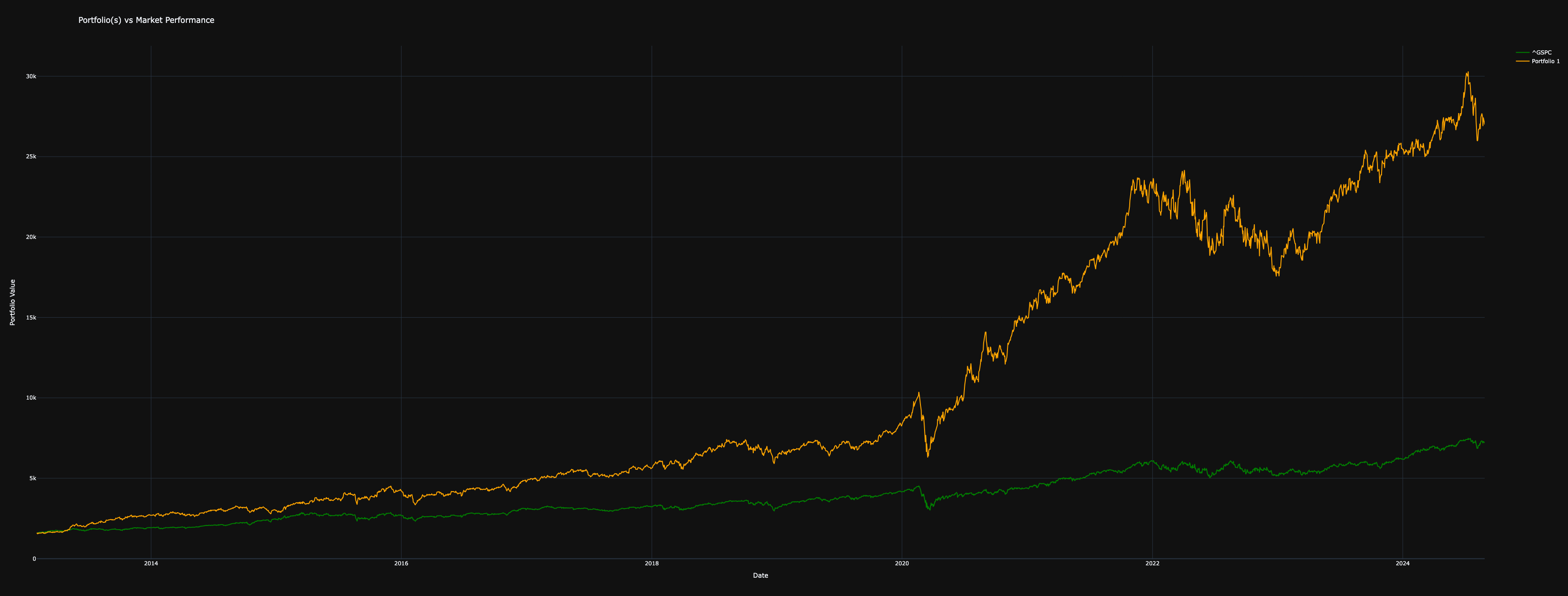
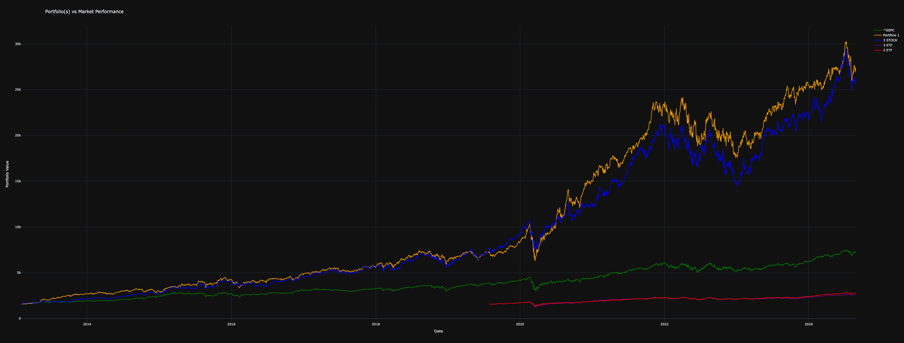
- Portfolio Value (
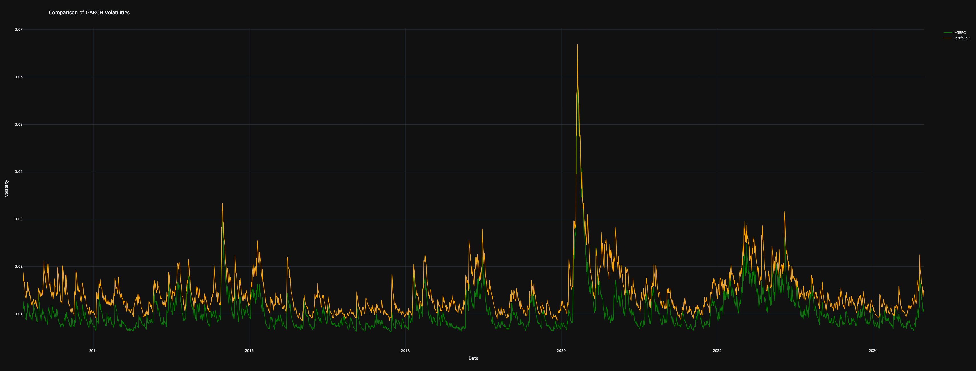
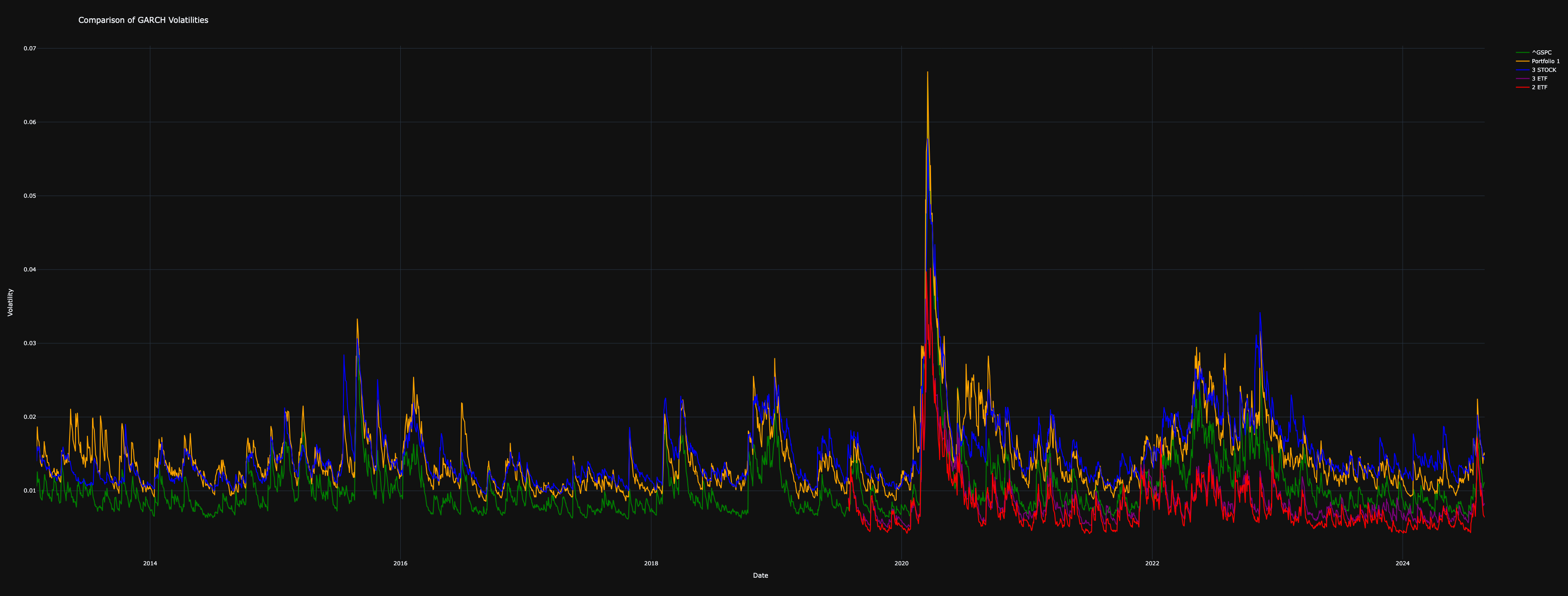
portfolio_value) – Compares portfolio performance against the market and visualizes portfolio growth. - GARCH Volatility (
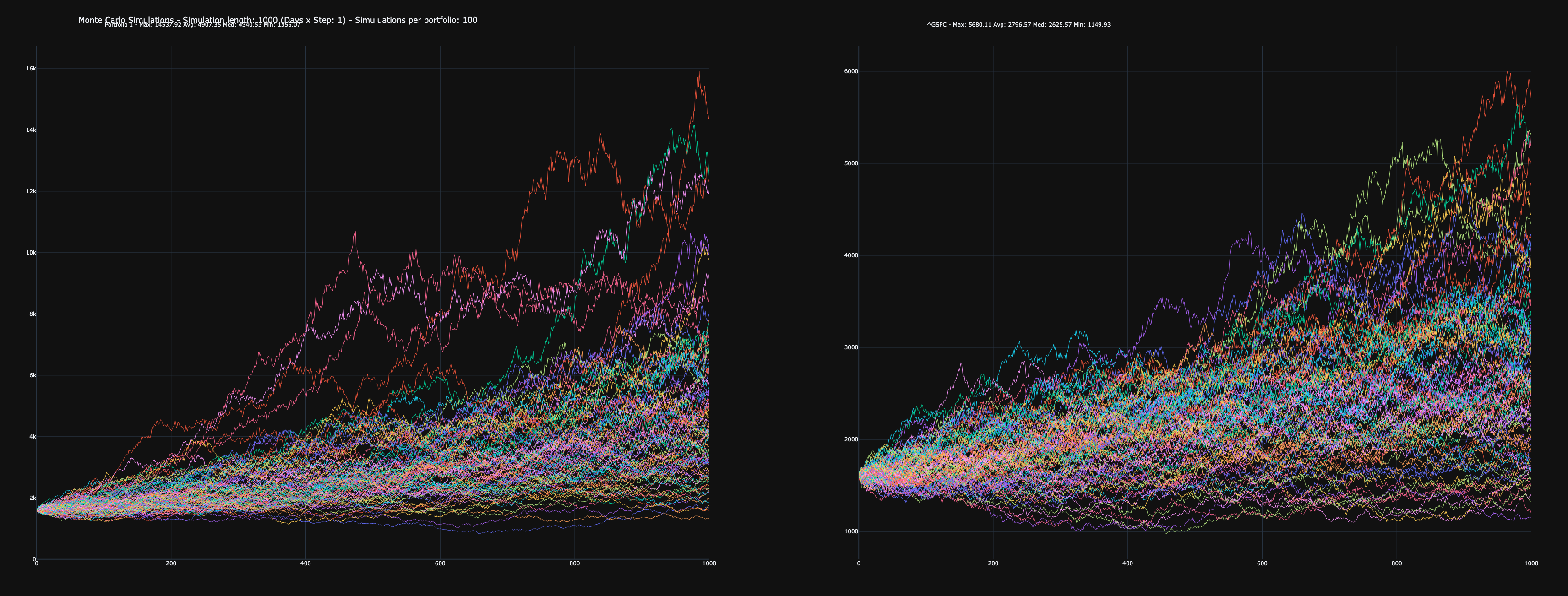
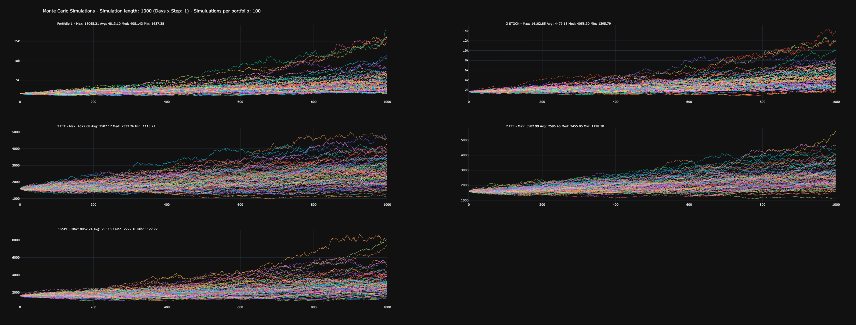
garch) – Estimates conditional volatility using a GARCH(1,1) model for risk assessment. - Monte Carlo Simulation (
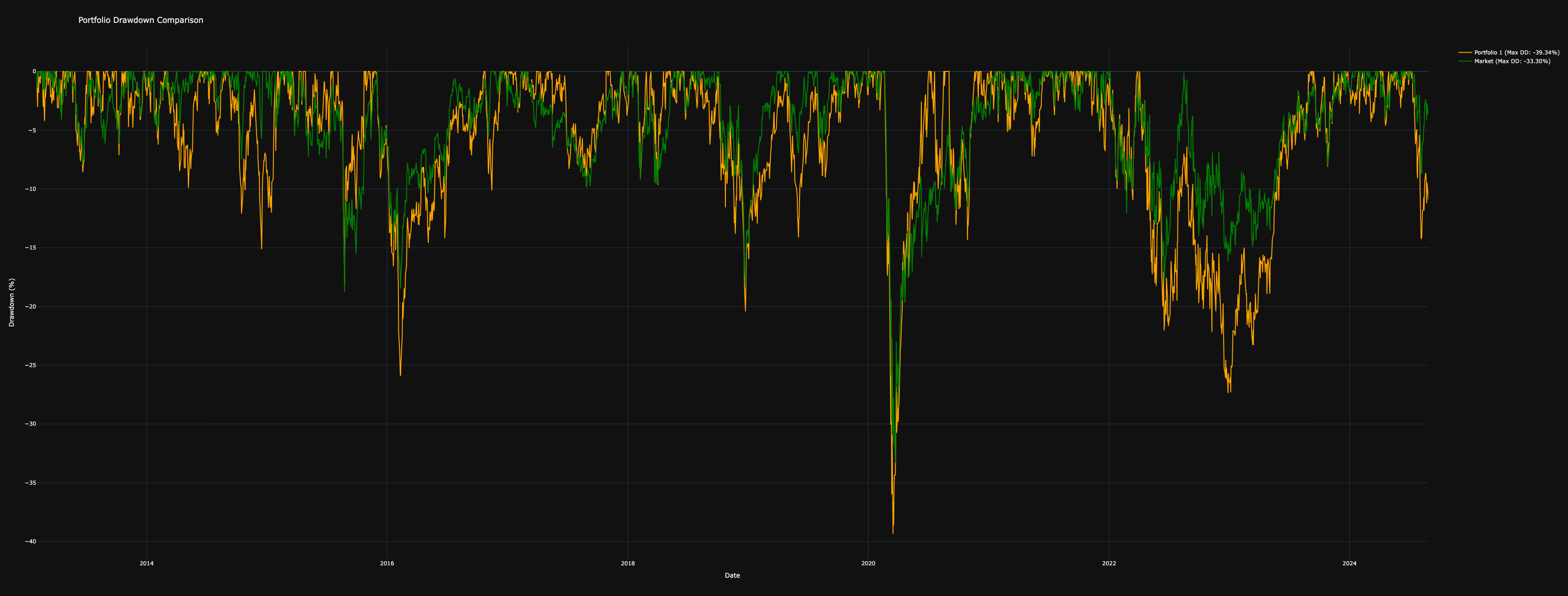
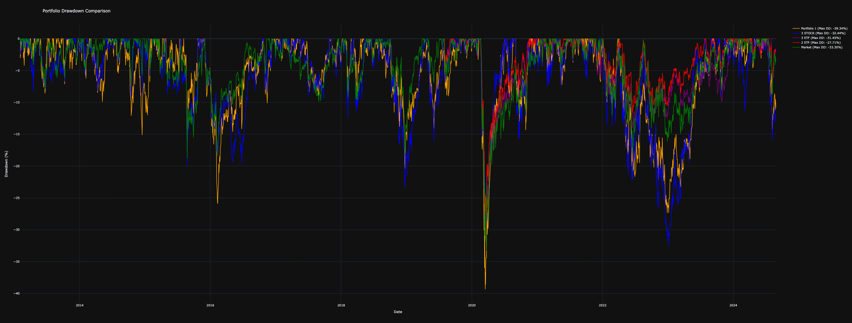
montecarlo) – Simulates future portfolio values based on historical returns. - Drawdown Analysis (
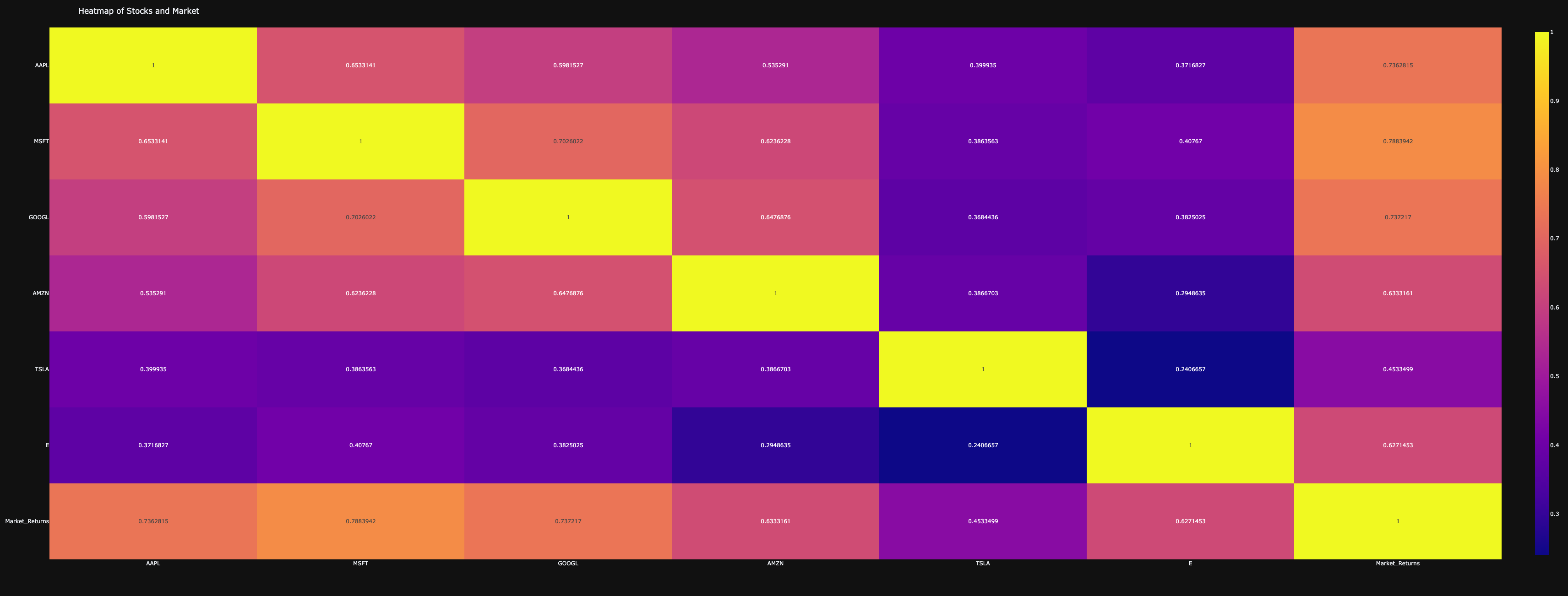
drawdown) – Calculates and visualizes maximum drawdowns over time. - Correlation Heatmap (
heatmap) – Generates a heatmap of correlations between portfolios or individual assets. - Asset Allocation (
pie_chart) – Visualizes portfolio allocation across assets in a pie chart. - Sector Distribution (
sector_pie) – Analyzes and plots the sector exposure of the portfolio. - Geographical Exposure (
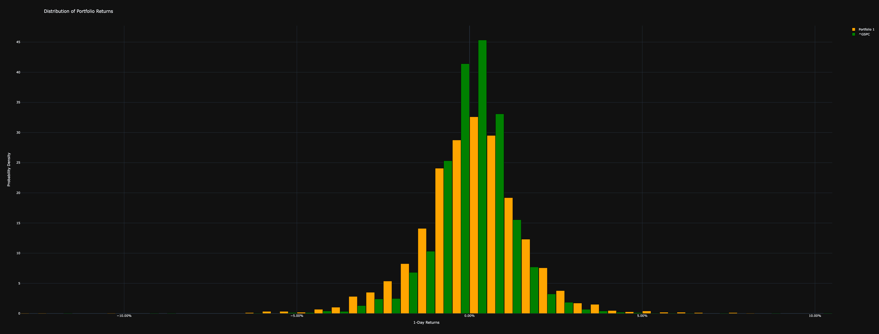
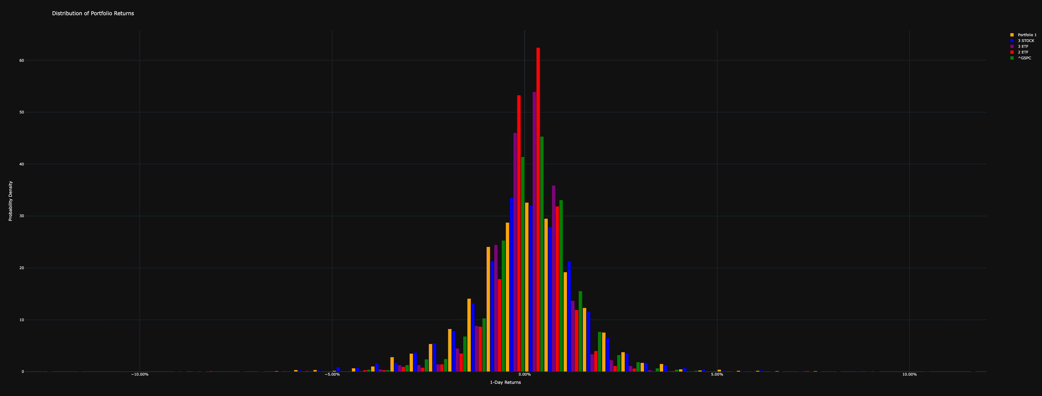
country_pie) – Displays the country distribution of portfolio assets. - Return Distribution (
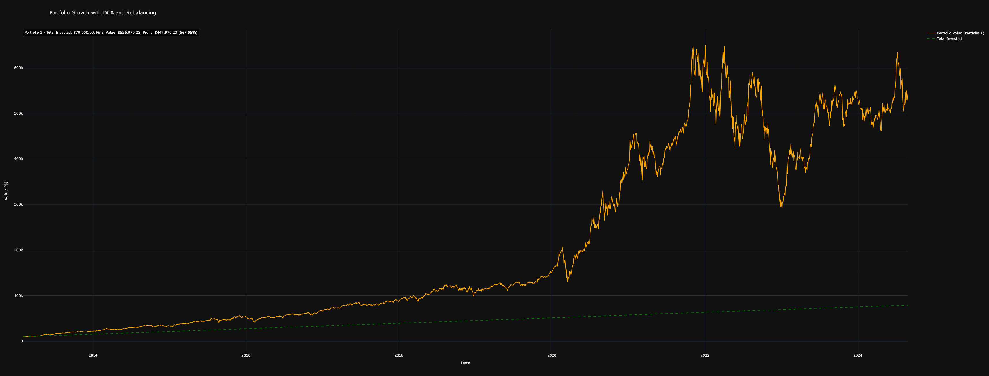
distribution_return) – Plots the histogram of portfolio returns to assess risk and performance. - Dollar-Cost Averaging Simulation (
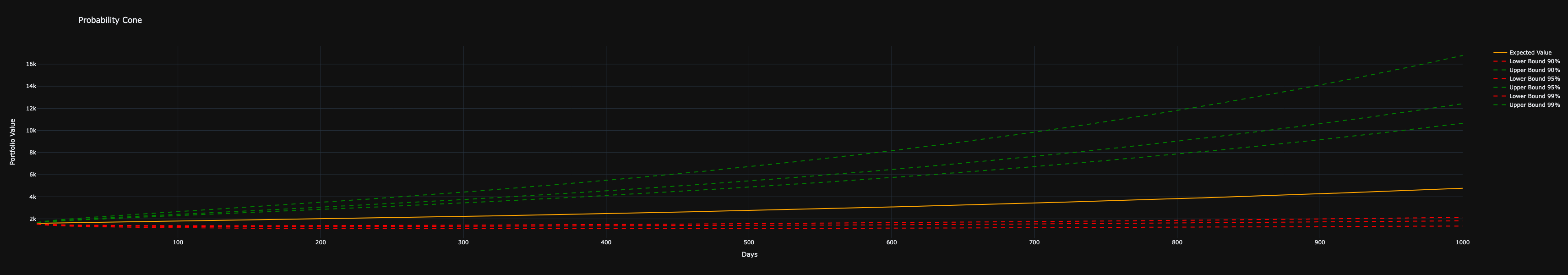
simulate_dca) – Models a periodic investment strategy with optional rebalancing. - Probability Cone (
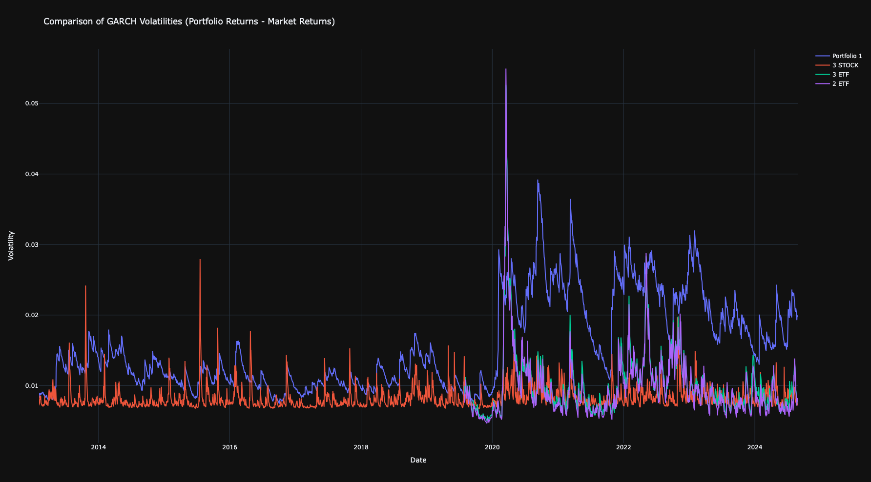
probability_cone) – Projects future portfolio values within confidence intervals. - GARCH Differential Volatility (
garch_diff) – Compares the volatility difference between portfolio returns and market returns.
Example: Graphics Module
colors_1 = "orange" #OPTIONAL
colors_4 = ["orange","blue","purple","red"] #OPTIONAL
start_date = '2013-02-01'
end_date = '2024-08-28'
market_ticker = '^GSPC'
base_currency = 'EUR'
risk_free = "DTB3"
ticker = ['AAPL','MSFT','GOOGL','AMZN','TSLA','E']
investments = [100,200,300,300,200,500]
data = ap.download_data(tickers=ticker, start_date=start_date, end_date=end_date, base_currency=base_currency,market_ticker=market_ticker, risk_free=risk_free)
portfolio_1 = ap.create_portfolio(data, ticker, investments, market_ticker=market_ticker, name_portfolio="Portfolio 1", base_currency=base_currency, rebalancing_period_days=250)
ticker = ['AAPL','MSFT','GOOGL']
investments = [500,300,800]
portfolio_2 = ap.create_portfolio(data, ticker, investments, market_ticker=market_ticker, name_portfolio="3 STOCK",base_currency=base_currency, rebalancing_period_days=250)
ticker = ["VWCE.DE","IGLN.L","IUSN.DE"]
investments = [500,300,800]
data = ap.download_data(tickers=ticker, start_date=start_date, end_date=end_date, base_currency=base_currency,market_ticker=market_ticker, risk_free=risk_free)
portfolio_3 = ap.create_portfolio(data, ticker, investments, market_ticker=market_ticker, name_portfolio="3 ETF", base_currency=base_currency, rebalancing_period_days=250)
ticker = ["VWCE.DE","IGLN.L"]
investments = [1300,300]
portfolio_4 = ap.create_portfolio(data, ticker, investments, market_ticker=market_ticker, name_portfolio="2 ETF",base_currency=base_currency, rebalancing_period_days=250)
ap.portfolio_value(portfolio_1, colors=colors_1)
ap.portfolio_value([portfolio_1,portfolio_2,portfolio_3,portfolio_4], colors=colors_4)
ap.garch(portfolio_1, colors=colors_1)
ap.garch([portfolio_1,portfolio_2,portfolio_3,portfolio_4], colors=colors_4)
ap.garch_diff([portfolio_1,portfolio_2,portfolio_3,portfolio_4])
ap.montecarlo(portfolio_1, simulation_length=1000)
ap.montecarlo([portfolio_1,portfolio_2,portfolio_3,portfolio_4], simulation_length=1000)
ap.drawdown(portfolio_1, colors=colors_1)
ap.drawdown([portfolio_1,portfolio_2,portfolio_3,portfolio_4], colors=colors_4)
ap.heatmap(portfolio_1)
ap.distribution_return(portfolio_1, colors=colors_1)
ap.distribution_return([portfolio_1,portfolio_2,portfolio_3,portfolio_4], colors=colors_4)
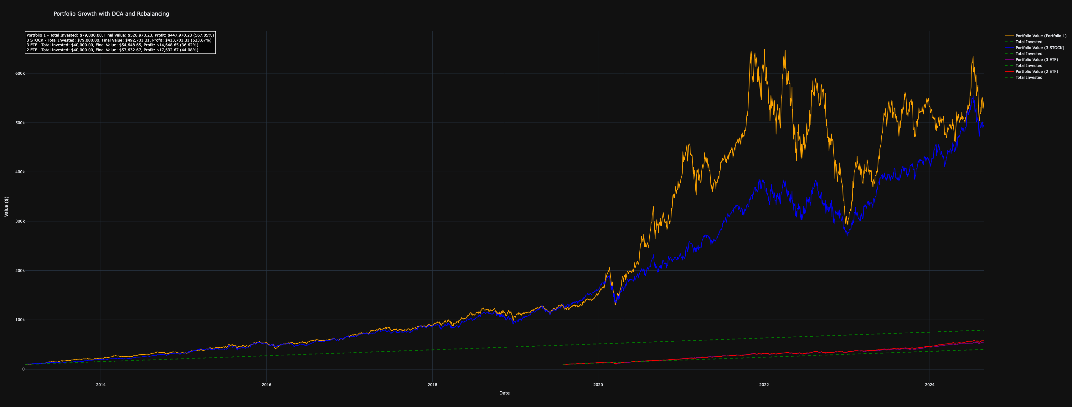
ap.simulate_dca(portfolio_1, initial_investment=10000, periodic_investment=500, investment_interval=30, colors=colors_1)
ap.simulate_dca([portfolio_1,portfolio_2,portfolio_3,portfolio_4], initial_investment=10000, periodic_investment=500, investment_interval=30, colors=colors_4)
ap.probability_cone(portfolio_1, time_horizon=1000)
Output Portfolio Value
Output Garch
Output Montecarlo
Output Drawdown
Output Heatmap
Output Distribution Returns
Output Simulate DCA
Output Probability Cone
Output Garch Diff
Optimization Module
- Portfolio Optimization (
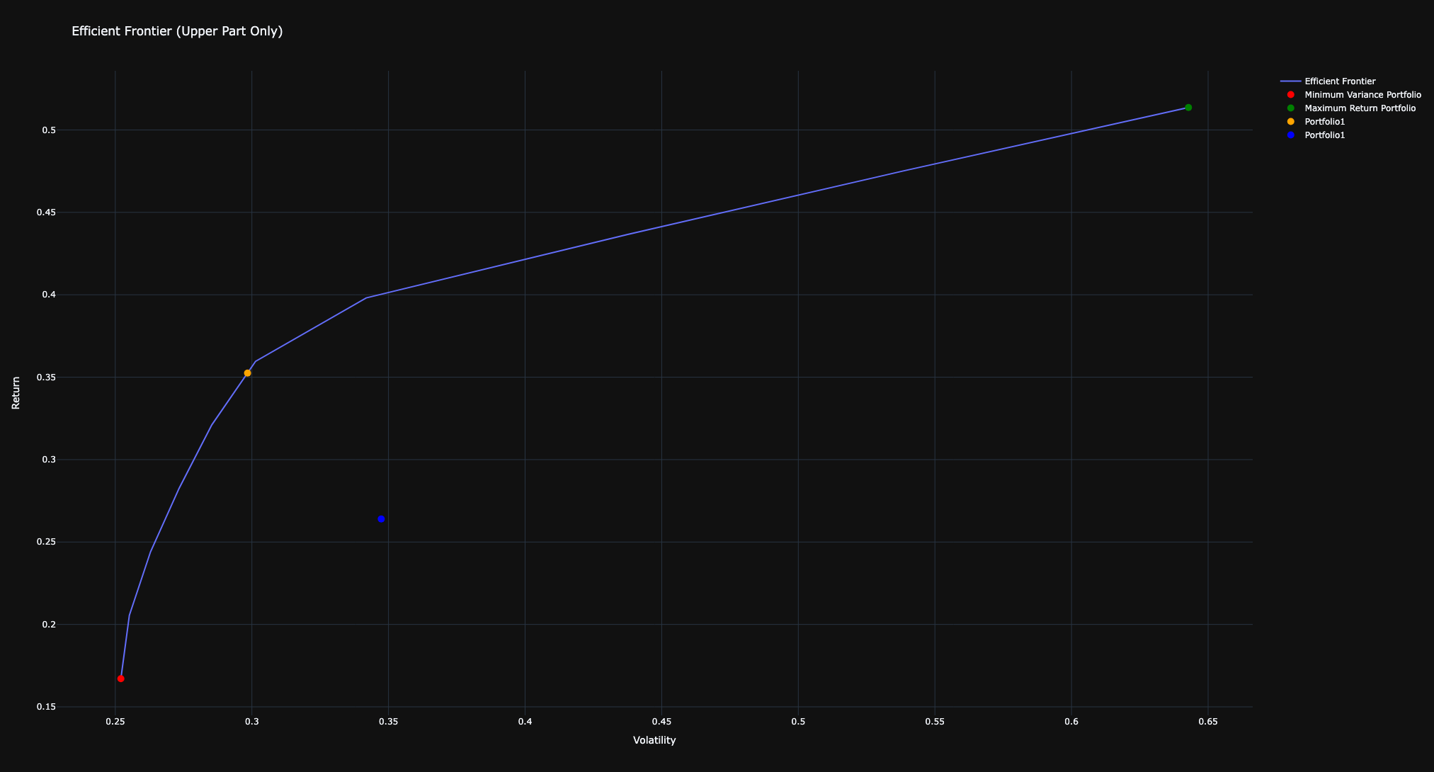
optimize) – Optimizes the portfolio allocation based on a chosen metric, such as Sharpe ratio, drawdown, volatility, or information ratio. - Efficient Frontier (
efficient_frontier) – Constructs and plots the efficient frontier, optimizing asset allocation to achieve various target returns while minimizing volatility.
Example: Optimization Module
sharpe=c_sharpe(portfolio_1)
portfolio_optimized=optimize(portfolio_1,metric='sharpe')
sharpe_optimized=c_sharpe(portfolio_optimized)

print("Sharpe ratio before optimization:",sharpe)
print("Sharpe ratio after optimization:",sharpe_optimized)

volatility1=c_volatility(portfolio_1)
portfolio_optimized=optimize(portfolio_1,metric='volatility')
volatility_optimized=c_volatility(portfolio_optimized)

print("Volatility before optimization:",volatility1)
print("Volatility after optimization:",volatility_optimized)

drawdown1=c_max_drawdown(portfolio_1)
portfolio_optimized=optimize(portfolio_1,metric='drawdown')
drawdown_optimized=c_max_drawdown(portfolio_optimized)

print("Max drawdown before optimization:",drawdown1)
print("Max drawdown after optimization:",drawdown_optimized)

information_ratio1=c_info_ratio(portfolio_1)
portfolio_optimized=optimize(portfolio_1,metric='information_ratio')
info_optimized=c_info_ratio(portfolio_optimized)

print("Information Ratio before optimization:",information_ratio1)
print("Information Ratio after optimization:",info_optimized)
Sharpe ratio before optimization:  0.7791344124615548
Sharpe ratio after optimization:  1.0963836499640336
Volatility before optimization:  0.3473494407821292
Volatility after optimization:  0.2520442151922823
Max drawdown before optimization:  0.5044136578460725
Max drawdown after optimization:  0.2896477982896617
Information Ratio before optimization:  0.5422909052526178
Information Ratio optimization:  1.1386493593167448
Output Efficient Frontier
efficient_frontier(portfolio_1,num_points=10, multi_thread=True, num_threads=3, additional_portfolios=[portfolio_optimized,portfolio_1], colors=["orange","blue"])
AI-Powered News Monitoring (monitor_news)
The monitor_news function enables real-time tracking of news for assets in a portfolio, leveraging Yahoo Finance as the news source. Additionally, it offers AI-driven news evaluation using OpenAI's GPT-4 to assess importance and sentiment.
Key Features
- Automated News Retrieval – Continuously fetches financial news for portfolio tickers from Yahoo Finance.
- AI-Powered Analysis (Optional) – Uses GPT-4 to evaluate the relevance and sentiment of each news article.
- Multi-Ticker Support – Avoids redundant checks and ensures efficient monitoring for all assets in the portfolio.
- Thread-Based Execution – Runs in the background, periodically fetching and analyzing news at user-defined intervals.
- Configurable Monitoring – Allows customization of monitoring frequency and whether the process runs indefinitely.
Parameters
portfolio (Union[Dict, List[Dict]])– Portfolio(s) containing tickers to monitor.openai_key (str, optional)– OpenAI API key for enabling GPT-4 news analysis. IfNone, only basic news retrieval is performed.delay (int, optional)– Frequency of news updates in seconds (default: 3600 seconds, i.e., 1 hour).loop_forever (bool, optional)– Whether the monitoring runs indefinitely (default: True).
Example: AI-Powered News Monitoring
# Start monitoring news with OpenAI analysis (Replace 'your-api-key' with an actual API key)
ap.monitor_news(portfolio, openai_key='your-api-key', delay=1800, loop_forever=True)
BMG - Bloomberg Data Downloader - UNDER TESTING
The bmg_download_data function enables efficient retrieval of historical financial data from Bloomberg Terminal, saving the results as CSV files. It supports multi-ticker downloads, currency conversion, and customizable data fields.
Features
- Automated Bloomberg Data Extraction – Fetch historical price data for multiple tickers.
- Currency Conversion – Retrieve prices in a specified base currency (default: USD).
- CSV Export – Save the downloaded data as CSV files for easy analysis.
- Customizable Fields – Specify the Bloomberg field to fetch (default:
last price).
Installation
Before using this function, ensure that Bloomberg Terminal is installed and running. Additionally, install the required Bloomberg Python API:
pip install --index-url=https://blpapi.bloomberg.com/repository/releases/python/simple/ blpapi
Example:
# Define parameters
tickers = ["AAPL US Equity", "MSFT US Equity"]
start_date = "2024-01-01"
end_date = "2024-02-01"
folder_path = "./data"
base_currency = "USD"
field = "last price"

# Download and save data
ap.bmg_download_data(tickers, start_date, end_date, folder_path, base_currency, field)
Logging & Plotly Customization
AnalyzerPortfolio allows users to configure logging and customize plotly visualizations to suit their needs. Below are the available customization options.
Logging Configuration
The logging system can be customized to control the level of detail, output location, and formatting of log messages.
Key logging functions
-
configure_logging:- Configures the logging behavior for the package.
- Parameters:
level(int): Overall logging level (e.g.,logging.INFO,logging.DEBUG).log_file(str, optional): Path to a file where logs will be saved. If not provided, logs will only be displayed in the console.console_level(int, optional): Specific logging level for the console. Defaults to the globallevel.verbose(bool, optional): IfTrue, console logs will display atDEBUGlevel.style(str, optional): Logging style. Options are:"detailed": Includes timestamps, levels, and logger names."print_like": Logs appear simple, like print statements.
Example:
configure_logging(level=logging.DEBUG, log_file="app.log", verbose=True, style="detailed")
-
reset_logging:- Resets the logging configuration by clearing all handlers.
- Useful if you want to reconfigure logging from scratch.
-
get_logger:- Retrieves the global logger for advanced configuration.
- Returns a
logging.Loggerinstance.
Plotly Configuration
AnalyzerPortfolio allows you to customize the appearance of Plotly visualizations by setting templates and transparency options.
Key Plotly functions
-
set_plotly_template:- Sets the global Plotly template and transparency option.
- Parameters:
template(str, optional): The name of the Plotly template to use. Default is"plotly_dark".transparent(bool, optional): IfTrue, the"transparent"template will be used, which makes the background transparent.
Example:
set_plotly_template(template="plotly_white", transparent=False)
-
get_plotly_template:- Retrieves the current global Plotly template.
- Returns the name of the active template as a
str.
Example:
template = get_plotly_template()
print(f"Current template: {template}")
-
is_transparent:- Checks if the transparent template is currently in use.
- Returns
Trueif the transparent template is active, otherwiseFalse.
Example:
if is_transparent():
    print("Transparent template is active")
Contributions
Contributions are welcome! Please submit pull requests or report issues via the GitHub repository.
Contacts


Download files
Download the file for your platform. If you're not sure which to choose, learn more about installing packages.
Source Distribution
Built Distribution
Filter files by name, interpreter, ABI, and platform.
If you're not sure about the file name format, learn more about wheel file names.
Copy a direct link to the current filters
File details
Details for the file analyzerportfolio-0.2.4.tar.gz.
File metadata
- Download URL: analyzerportfolio-0.2.4.tar.gz
- Upload date:
- Size: 53.8 kB
- Tags: Source
- Uploaded using Trusted Publishing? No
- Uploaded via: twine/6.1.0 CPython/3.10.5
File hashes
| Algorithm | Hash digest | |
|---|---|---|
| SHA256 |
fe9a5be98cc9856ea6bb6a9876d277c685d08f95181d6dcc19140b103acac277
|
|
| MD5 |
04058933375f21ce76807c825dfb098f
|
|
| BLAKE2b-256 |
1bac7d3da13d8df0f60c65264a9fed747a39603eabf1df4eb1bc4025ac7ee6ab
|
File details
Details for the file analyzerportfolio-0.2.4-py3-none-any.whl.
File metadata
- Download URL: analyzerportfolio-0.2.4-py3-none-any.whl
- Upload date:
- Size: 47.0 kB
- Tags: Python 3
- Uploaded using Trusted Publishing? No
- Uploaded via: twine/6.1.0 CPython/3.10.5
File hashes
| Algorithm | Hash digest | |
|---|---|---|
| SHA256 |
557a6527370f01dedc402b0cdc4f5e3d6fbf6f0fbfa3ded814b9f1f638c13a51
|
|
| MD5 |
9bee6dfca56c9405bc179a1a55e7dbe9
|
|
| BLAKE2b-256 |
e3a5394ed228c3b8a76c1310859c1a15904747f01fdc21241b734d808996b72f
|


