
Approximate Bayesian Computation Python Package
Package Description
Approximate Bayesian Computation (ABC) is a statistical method to fit a Bayesian model to data when the likelihood function is hard to compute.
The approxbayescomp package implements an efficient form of ABC — the sequential Monte Carlo (SMC) algorithm.
While it can handle any general statistical problem, we built in some models so that fitting insurance loss distributions is particularly easy.
The full documentation is available at https://pat-laub.github.io/approxbayescomp.
Installation
To install simply run
pip install approxbayescomp
Example
Using a built-in data generating process simulation method
Consider a basic insurance example where each month our insurance company receives a random number of claims, each of which is of a random size. Specifically, say that in month $i$ we have $N_i \sim \mathsf{Poisson}(\lambda)$ i.i.d. number of claims, and each claim is $U_{i,j} \sim \mathsf{Lognormal}(\mu, \sigma^2)$ sized and i.i.d. At each month we can observe the aggregate claims, that is, $X_i = \sum_{j=1}^{N_i} U_{i,j}$ for $i=1,\dots,T$, that is, we observe $T$ months of data. Lastly, we have the prior beliefs that $\lambda \sim \mathsf{Unif}(0, 100),$ $\mu \sim \mathsf{Unif}(-5, 5),$ and $\sigma \sim \mathsf{Unif}(0, 3).$
The approxbayescomp code to fit this data would be:
import approxbayescomp as abc

# Load data to fit (modify this line to load real observations!)
obsData = [1.0, 2.0, 3.0]

# Specify our prior beliefs over (lambda, mu, sigma).
prior = abc.IndependentUniformPrior([(0, 100), (-5, 5), (0, 3)])

# Fit the model to the data using ABC
model = abc.Model("poisson", "lognormal", abc.Psi("sum"))
numIters = 6  # The number of SMC iterations to perform
popSize = 250  # The population size of the SMC method

fit = abc.smc(numIters, popSize, obsData, model, prior)
Then fit will contain a collection of weighted samples from the approximate posterior distribution of $(\lambda, \mu, \sigma)$.
The posterior mean for these parameters would be easily calculated:
import numpy as np

print("Posterior mean of lambda: ", np.sum(fit.samples[:, 0] * fit.weights))
print("Posterior mean of mu: ", np.sum(fit.samples[:, 1] * fit.weights))
print("Posterior mean of sigma: ", np.sum(fit.samples[:, 2] * fit.weights))
Using a user-suppled simulation method
We have built many standard insurance loss models into the package, so in the previous example
model = abc.Model("poisson", "lognormal", abc.Psi("sum"))
is all that is required to specify this data-generating process. However, for non-insurance processes, we have to supply a function to simulate from the data-generating process. The equivalent version for this example would be:
import numpy.random as rnd

def simulate_aggregate_claims(theta, T):
    """
    Generate T observations from the model specified by theta.
    """
    lam, mu, sigma = theta
    freqs = rnd.poisson(lam, size=T)
    aggClaims = np.empty(T, np.float64)
    for t in range(T):
        aggClaims[t] = np.sum(rnd.lognormal(mu, sigma, size=freqs[t]))
    return aggClaims

simulator = lambda theta: simulate_aggregate_claims(theta, len(obsData))
fit = abc.smc(numIters, popSize, obsData, simulator, prior)
Modifying just these lines will be equivalent to the example above. Note the output won't be identical since (in this case) the two alternatives use different random number generation techniques (numba vs numpy).
Other Examples and Resources
See the What is ABC page for an illustrative example of the core ABC concept. For examples of this package in use, start with the Geometric-Exponential example page and the following ones.
This package is the result of our paper "Approximate Bayesian Computation to fit and compare insurance loss models". For a detailed description of the aims and methodology of ABC check out this paper. It was written with ABC newcomers in mind.
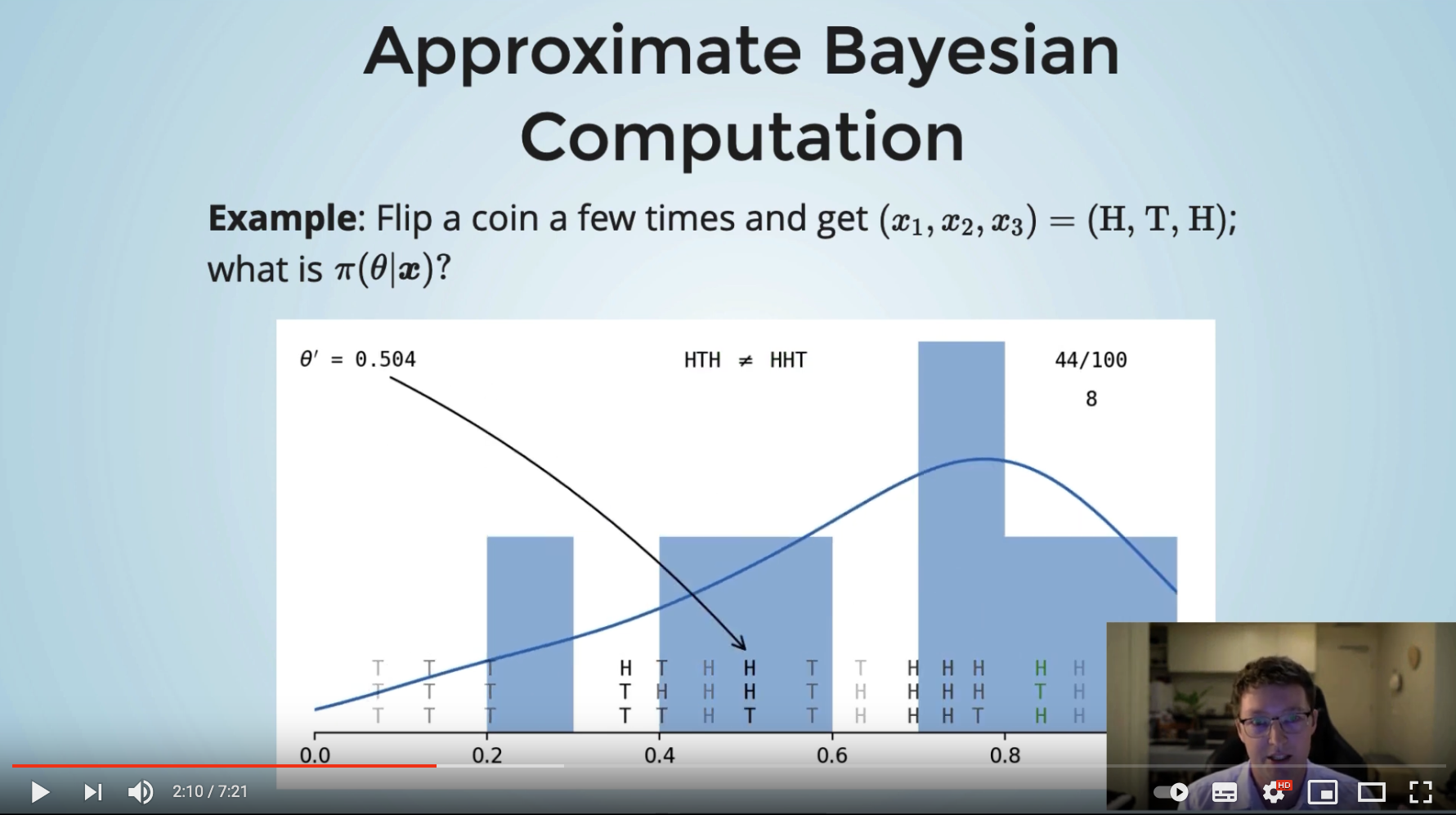
If you prefer audio/video, see Patrick's 7 min lightning talk at the Insurance Data Science conference:
Details
The main design goal for this package was computational speed.
ABC is notoriously computationally demanding, so we spent a long time optimising the code as much as possible.
The key functions are JIT-compiled to C with numba (we experimented with JIT-compiling the entire SMC algorithm, but numba's random variable generation is surprisingly slower than numpy's implementation).
Everything that can be numpy-vectorised has been.
And we scale to use as many CPU cores available on a machine using joblib.
We also aimed to have total reproducibility, so for any given seed value the resulting ABC posterior samples will always be identical.
Our main dependencies are joblib, numba, numpy, and scipy. Also, the package sometimes calls functions from matplotlib, tqdm, and hilbertcurve.
Note, Patrick has a rough start at a C++ version of this package at the cppabc repository. It only handles the specific Geometric-Exponential random sums case, though if you are interested in collaborating to expand this, let him know!
Authors
- Patrick Laub (author, maintainer),
- Pierre-Olivier Goffard (author).
Citation
Pierre-Olivier Goffard, Patrick J. Laub (2021), Approximate Bayesian Computations to fit and compare insurance loss models, Insurance: Mathematics and Economics, 100, pp. 350-371
@article{approxbayescomp,
  title={Approximate Bayesian Computations to fit and compare insurance loss models},
  author={Goffard, Pierre-Olivier and Laub, Patrick J},
  journal={Insurance: Mathematics and Economics},
  volume={100},
  pages={350--371},
  year={2021}
}
1 maintainer

Metadata
1 maintainer
Release files for approxbayescomp 0.2.1
For a detailed explanation of source distributions (sdists) and built distributions (wheels), please see the package formats documentation.
Source distribution (sdist)
| File | Size | Uploaded | |
|---|---|---|---|
| approxbayescomp-0.2.1.tar.gz | 33.1 kB | Details |
Built distribution (wheel)
| File | Interpreter | ABI | Platform | Reset |
|---|---|---|---|---|
| approxbayescomp-0.2.1-py3-none-any.whl | Python 3 | none | any | Details |
Total release size: 64.4 kB
Release files / approxbayescomp-0.2.1.tar.gz
| Download URL | approxbayescomp-0.2.1.tar.gz |
|---|---|
| Size | 33.1 kB |
| Tags | Source |
|
SHA-256 checksum How to use checksums |
eeae513d82fa30d60c4c9eb6672b6535acc4152392676a05dd17da738f0ea8f3
|
|
BLAKE2b-256 checksum How to use checksums |
3b2e8ed920a79ab03c94cd7e027d8337913f3e241fbdb77f94addbe8e458ee98
|
| Upload date | |
|
Uploaded using Trusted Publishing? What is trusted publishing? |
No |
| Uploaded via |
twine/4.0.2 CPython/3.11.6
|
Release files / approxbayescomp-0.2.1-py3-none-any.whl
| Download URL | approxbayescomp-0.2.1-py3-none-any.whl |
|---|---|
| Size | 31.3 kB |
| Tags | Python 3 |
|
SHA-256 checksum How to use checksums |
f58b49ba92d3e520a007cbdb14ffa531f61ef8ae5a4a1371003a74bbd3fabbf8
|
|
BLAKE2b-256 checksum How to use checksums |
f493f7fb8681ea6e4658d7785e1026fe14414a1d212dcbffa50ba362c4954ed5
|
| Upload date | |
|
Uploaded using Trusted Publishing? What is trusted publishing? |
No |
| Uploaded via |
twine/4.0.2 CPython/3.11.6
|














