
arbital





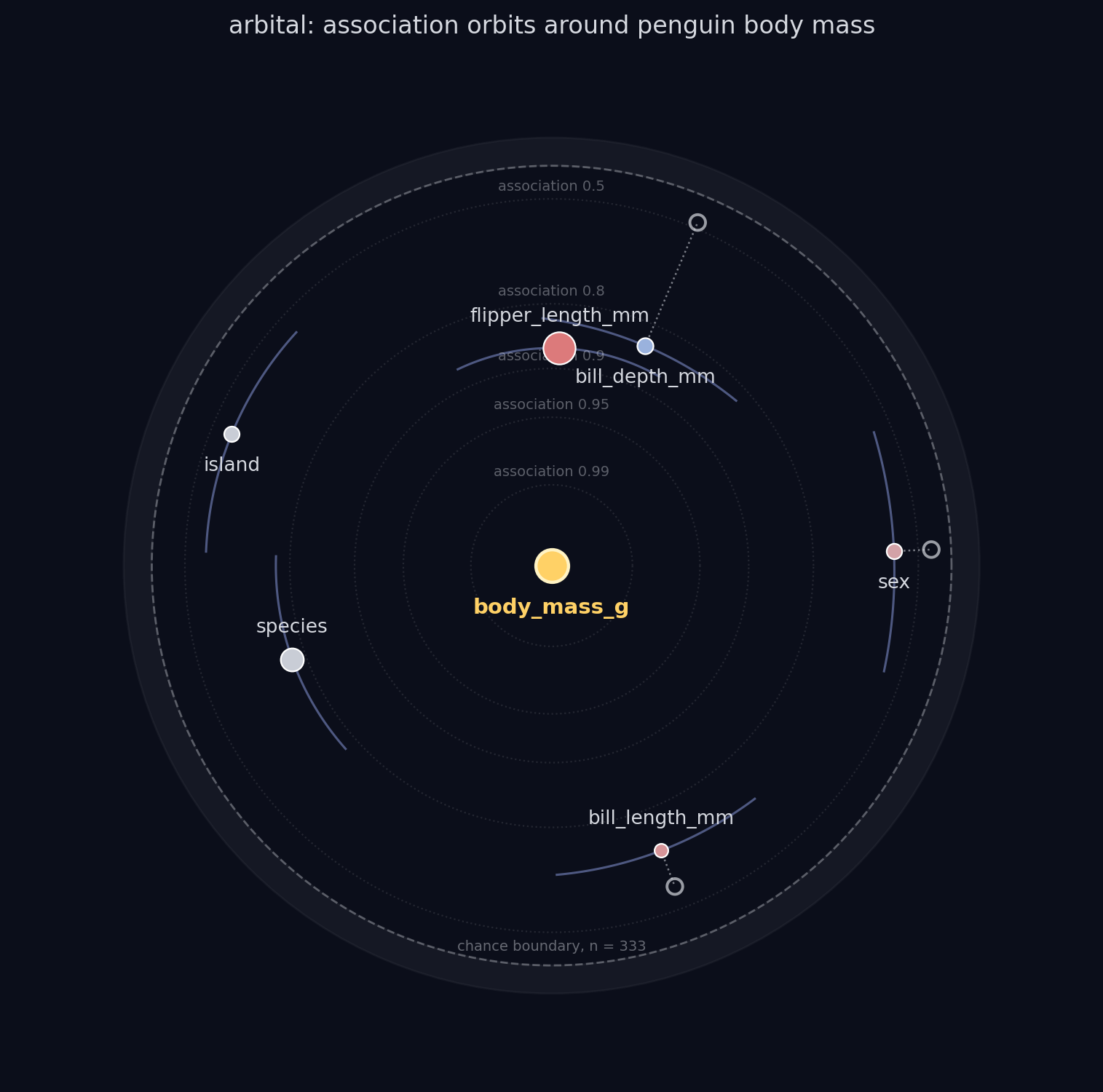
arbital draws every variable in a dataset as an orbit around a target, so that the strength, shape, direction, redundancy, and usefulness of each association are readable from a single figure.
Why correlation fails
The first look at a new dataset is almost always a correlation matrix, and a correlation matrix can only see straight lines (or, for rank correlation, monotone curves). Three common structures defeat it entirely:
- Non-monotone relationships. A parabola or a sine wave has r ≈ ρ ≈ 0. A correlation screen ranks it with the noise and discards it.
- Interactions. If y = x₁·x₂, each parent is individually uncorrelated with y, since the other parent randomly flips the sign of its effect, yet y is strongly dependent on both.
- Pooled groups (Simpson's paradox). In the Palmer penguins data, bill depth versus body mass has r = −0.47 pooled across species, while the relationship is positive within every species. The correlation is not just weak; its sign is wrong.
Mutual information detects all three, but raw mutual information is expressed in nats, has no upper bound in common use, and is painful to read in bulk. So in practice it rarely replaces the correlation matrix as the first look.
What arbital adds
arbital (Association Radii By Information-Theoretic Association Learning) measures every variable against the target with both families of statistics and encodes the comparison geometrically:
| Element | Meaning |
|---|---|
| radius | total association with the target, logarithmic in mutual information (closer is stronger) |
| ghost marker + tether | where correlation alone would place the variable, and the association it misses |
| orbit eccentricity | the nonlinear share ν (a circle is a purely monotone relationship) |
| angle | associated variables huddle together; a tight cluster is a redundant group, a lone variable carries independent information |
| marker size | marginal gain under greedy mRMR feature selection by default (largest = strong and non-redundant); switch to total association or a constant with size="rinfo"/"uniform" |
| colour | direction of the relationship (signed Spearman ρ; neutral for nominal categories) |
The figure is interactive (Plotly), and every quantity in it is available as a plain table.
Five lines
import arbital
from arbital import datasets

cars = datasets.load_mpg()                          # bundled, loads offline
arbital.orbits(cars, target="mpg").to_html("mpg.html")
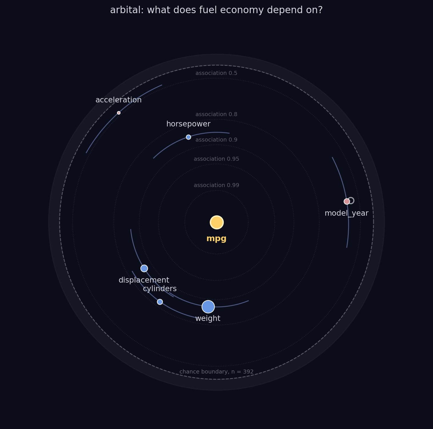
Weight, displacement, cylinders and horsepower huddle in one angular sector, one redundant
engine-size group, of which the selection keeps only weight (largest marker), while
model_year sits alone: weaker individually, but independent information.
Installation
pip install arbital                                    # from PyPI (core: NumPy only)
pip install git+https://github.com/aaronbyrnephd/arbital   # latest from GitHub
pip install "arbital[plotly,datasets]"                 # optional extras
For development: clone, pip install -e ".[test]", pytest tests/.
The core package depends only on NumPy. to_html() needs no plotly install (it emits Plotly
JSON plus a CDN script); the plotly extra is only for live Figure objects. Four example
datasets (mpg, penguins, titanic, tips) are bundled and load offline; with the datasets
extra, datasets.load("<name>") fetches any of seaborn's ~20 bundled datasets by name
(diamonds, iris, planets, taxis, flights, ...); datasets.available() lists them all.
Quick start
import arbital
from arbital import datasets

cars = datasets.load_mpg()            # or datasets.load("<any seaborn dataset>")
space = arbital.orbits(cars, target="mpg")
space.to_html("mpg.html")             # standalone interactive figure
space.table()                         # per-feature metrics as dicts
space.to_df()                         # the same as a pandas DataFrame
space.selection()                     # the greedy mRMR walkthrough, one dict per pick

# feature selection on its own, without a figure:
arbital.select_features(cars, target="mpg")

# don't know the target yet? let arbital suggest one:
arbital.select_target(cars)           # index of the column most associated with the rest

# categorical target and fields, with bootstrap uncertainty arcs:
arbital.orbits(datasets.load_titanic(), target="survived",
               selection=True, uncertainty=True)
Any 2-D NumPy array or object exposing .columns and array semantics (including a pandas
DataFrame) is accepted; string columns are detected as categorical and rows with missing
values are dropped.
Features
- One bounded scale for everything. Mutual information is converted to Linfoot's informational coefficient r_I ∈ [0, 1), directly comparable with |r| and |ρ|.
- Mixed data types. Continuous, categorical, and mixed pairs each get the appropriate mutual-information estimator, selected automatically.
- Honest feature selection, three ways to look at it. Greedy mRMR with r_I as both
relevance and redundancy; marginal gains are recorded at pick time. Run it standalone with
select_features(), get the full walkthrough (relevance, redundancy, gain per pick) fromOrbitSystem.selection(), or just number the markers in the figure withselection=True. - Chance-calibrated selection, without moving the plot. Finite-sample k-NN estimators
report small positive MI even for independent pairs; arbital measures that chance level
against shuffled copies of the target and draws it as a boundary circle to compare markers
against directly. Feature selection ranks on a separately chance-subtracted relevance, so
unassociated features score zero and cannot win a pick. r_info itself, and every
marker's position, is always the estimated value (calibrating both would double-count
chance against the same boundary). Pearson and Spearman get the same treatment
(
pearson_sig/spearman_sig) from the same permutation draws and the sameconfidence(default 0.95, one tunable parameter for every channel), a different, complementary question from whether r_info clears chance, not a differently-calibrated one.calibrate=Falseskips all of it. This is a heuristic screen, not a rigorous test: no multiple-comparison correction is applied across the features you screen at once, and the vignette's Assumptions and calibration caveats section lists every place this trades statistical rigor for a usable default. - Uncertainty on demand.
uncertainty=Truebootstraps a standard error for every r_info and draws it as a radial band through the marker; a diamond flags bands that cross the chance boundary (that association could be noise). - Meaningful angles. Three layouts:
"spread"(default; embedding gaps with a readable minimum separation),"embed"(raw embedding),"ordered"(even spacing). - Auto target.
target=Nonepicks the variable the rest of the data revolves around (select_target()is the same logic, usable on its own before you've decided what to plot). - Light by design. Pure-NumPy estimators you can read in one sitting; no compiled
extensions; figures as plain JSON. Rows are subsampled beyond
max_samples=2000because the k-NN estimator is O(n²); all estimators take a seed for reproducibility.
Documentation
- Usage vignette: the full tour, synthetic
ground truth, redundancy groups and the angle axis, transformed and lagged variables,
interactions, categorical data, Simpson's paradox, selection, uncertainty, and a glossary of
every quantity the hover/table/
to_df()report. Published on every push tomain; also downloadable from the repo. - API reference: every public function
and class, generated from the docstrings below with pdoc; the same
content
help(arbital.orbits)gives you at a prompt, browsable. - Tutorial notebook: hands-on version of the vignette.
- Repository layout:
src/arbital/measures.py(estimators),geometry.py(orbit mapping, layout, selection),plot.py(Plotly JSON),datasets.py(bundled data),tests/(property-based suite),demo/(vignette builder).
See CONTRIBUTING.md to get involved and RELEASING.md for the release process.
Theory
Mutual information I(x;y) is estimated per pair: Kraskov–Stögbauer–Grassberger k-nearest neighbour for continuous pairs, Ross's estimator for continuous–categorical, and a plug-in estimator for categorical pairs. It is placed on the correlation scale with Linfoot's
r_I = √(1 − e^(−2I)),
which equals |ρ| exactly for a bivariate Gaussian. The Gaussian statement is a calibration, not an assumption: r_I is a fixed monotone transform of mutual information, so it ranks variables identically to MI for any distribution, is zero under independence, approaches 1 as the relationship becomes deterministic, and (for continuous pairs) depends only on the copula, since mutual information there is exactly the negative entropy of the copula density (Joe, 1989). The radius is the residual uncertainty
d = √(1 − r_I²) = e^(−I),
so the radial axis is logarithmic in information: every factor of e closer to the centre is one more nat. The orbit's eccentricity is the nonlinear share
ν = 1 − (r_mono / r_I)², with r_mono = max(|r|, |ρ|),
the fraction of total dependence a monotone description misses (ν is a composite defined for this package, not a standard named statistic). The periastron of each orbit sits at d(r_I), the apastron at d(r_mono), so the ghost/tether is ν drawn to scale. Angles come from classical MDS on the feature–feature r_I matrix; marker sizes from greedy mRMR selection; uncertainty arcs from a nonparametric bootstrap.
References
- Pearson, K. (1895). Notes on regression and inheritance in the case of two parents. Proceedings of the Royal Society of London, 58, 240–242. (Pearson r)
- Spearman, C. (1904). The proof and measurement of association between two things. American Journal of Psychology, 15(1), 72–101. (Spearman ρ)
- Shannon, C. E. (1948). A mathematical theory of communication. Bell System Technical Journal, 27, 379–423. (mutual information)
- Torgerson, W. S. (1952). Multidimensional scaling: I. Theory and method. Psychometrika, 17(4), 401–419. (classical MDS for the angular layout)
- Linfoot, E. H. (1957). An informational measure of correlation. Information and Control, 1(1), 85–89. (the r_I scale)
- Efron, B. (1979). Bootstrap methods: another look at the jackknife. The Annals of Statistics, 7(1), 1–26. (uncertainty arcs)
- Joe, H. (1989). Relative entropy measures of multivariate dependence. Journal of the American Statistical Association, 84(405), 157–164. (r_I depends only on the copula)
- Kraskov, A., Stögbauer, H., & Grassberger, P. (2004). Estimating mutual information. Physical Review E, 69(6), 066138. (KSG estimator, continuous pairs)
- Peng, H., Long, F., & Ding, C. (2005). Feature selection based on mutual information: criteria of max-dependency, max-relevance, and min-redundancy. IEEE Transactions on Pattern Analysis and Machine Intelligence, 27(8), 1226–1238. (mRMR)
- Ross, B. C. (2014). Mutual information between discrete and continuous data sets. PLoS ONE, 9(2), e87357. (mixed continuous–categorical estimator)
License and citation
MIT, see LICENSE. If you use arbital in research, see CITATION.cff (GitHub's "Cite this
repository" button).
1 maintainer

Release files for arbital 0.1.3
For a detailed explanation of source distributions (sdists) and built distributions (wheels), please see the package formats documentation.
Source distribution (sdist)
| File | Size | Uploaded | |
|---|---|---|---|
| arbital-0.1.3.tar.gz | 75.7 kB | Details |
Built distribution (wheel)
| File | Interpreter | ABI | Platform | Reset |
|---|---|---|---|---|
| arbital-0.1.3-py3-none-any.whl | Python 3 | none | any | Details |
Total release size: 134.3 kB
Release files / arbital-0.1.3.tar.gz
| Download URL | arbital-0.1.3.tar.gz |
|---|---|
| Size | 75.7 kB |
| Tags | Source |
|
SHA-256 checksum How to use checksums |
1a982697308da84a8aa628ef423d1e4cfecf0a682d13f8cb1a824d2263184ae6
|
|
BLAKE2b-256 checksum How to use checksums |
932059dfef36f1b3cbcb9a5867d0f67f6c7e4db7d0cf4522757b01a1318114f1
|
| Upload date | |
|
Uploaded using Trusted Publishing? What is trusted publishing? |
Yes |
| Uploaded via |
twine/7.0.0 CPython/3.13.14
|
Provenance
Provenance describes where a file came from. On PyPI, provenance is shared via attestations, which provide a verifiable record of the build or publishing details. View details, limitations and caveats.


PyPI Publish Attestation
PyPI verified that this artifact, at this checksum, originated from the publisher listed below.
Signed by GitHub Actions, verified by PyPI on Aug 8, 2026.
Transparency logRelease files / arbital-0.1.3-py3-none-any.whl
| Download URL | arbital-0.1.3-py3-none-any.whl |
|---|---|
| Size | 58.5 kB |
| Tags | Python 3 |
|
SHA-256 checksum How to use checksums |
fe6e99cb7c8d59298735297d86a60eedd7062d4c84e246311a03afd8ba9c508c
|
|
BLAKE2b-256 checksum How to use checksums |
383af0b56029075532da43c0bbd0225d7b10396625eab027d7e05bf61c77661d
|
| Upload date | |
|
Uploaded using Trusted Publishing? What is trusted publishing? |
Yes |
| Uploaded via |
twine/7.0.0 CPython/3.13.14
|
Provenance
Provenance describes where a file came from. On PyPI, provenance is shared via attestations, which provide a verifiable record of the build or publishing details. View details, limitations and caveats.
PyPI Publish Attestation
PyPI verified that this artifact, at this checksum, originated from the publisher listed below.
Signed by GitHub Actions, verified by PyPI on Aug 8, 2026.
Transparency log













