
Conditional inference trees for Python

Project description
Sigma

Conditional inference trees for Python.
Provides classification (ClassificationTree), regression
(RegressionTree), survival-analysis (SurvivalTree), and ranking
(RankingTree) estimators, compatible with scikit-learn.
- Unbiased splits - permutation-based p-values decouple variable selection from split search, avoiding CART's bias toward variables with many possible splits
- Interpretable by construction - each split is a statistical hypothesis test with a reported p-value, and fitted trees render to PNG, PDF, SVG, or GIF via
to_image - scikit-learn compatible -
ClassificationTree,RegressionTree,SurvivalTree, andRankingTreedrop into any sklearn pipeline
Every statistical method in Sigma comes from a peer-reviewed paper.
1. License
Governed by the Sigma License. This is a source-available license, not OSI-approved open source. Commercial use is permitted with attribution. ArsChitectura SAS retains an at-will right to revoke the license, at any time, for any reason. Licensee shall consult Licensor's organization website and the Software's project homepage at least once every ninety (90) days.
AI, ML, and other automated ingestion of this library, its documentation, or any derivative work is prohibited, excepted to generate your own client code that calls Sigma's public API.
Modification of Sigma is permitted only as preparation for a Contribution
to the Canonical Repository; see CONTRIBUTING.md
for the lifecycle.
External contributors must sign the CLA in CONTRIBUTING.md
before a pull request can be accepted.
If your needs exceed this, a paid, non-revocable commercial license is available on request.
2. Support
Read the documentation.
Have questions, feedback, or need help getting started? I would love to hear from you - get in touch.

3. Installation
pip install ars-sigma
4. Sample Trees
Four trees fitted on classic datasets. Each subsection shows the
fit code, the to_text rendering, and the rendered tree and response
images. Click an image to view it at full size.
4.1. Titanic (classification)
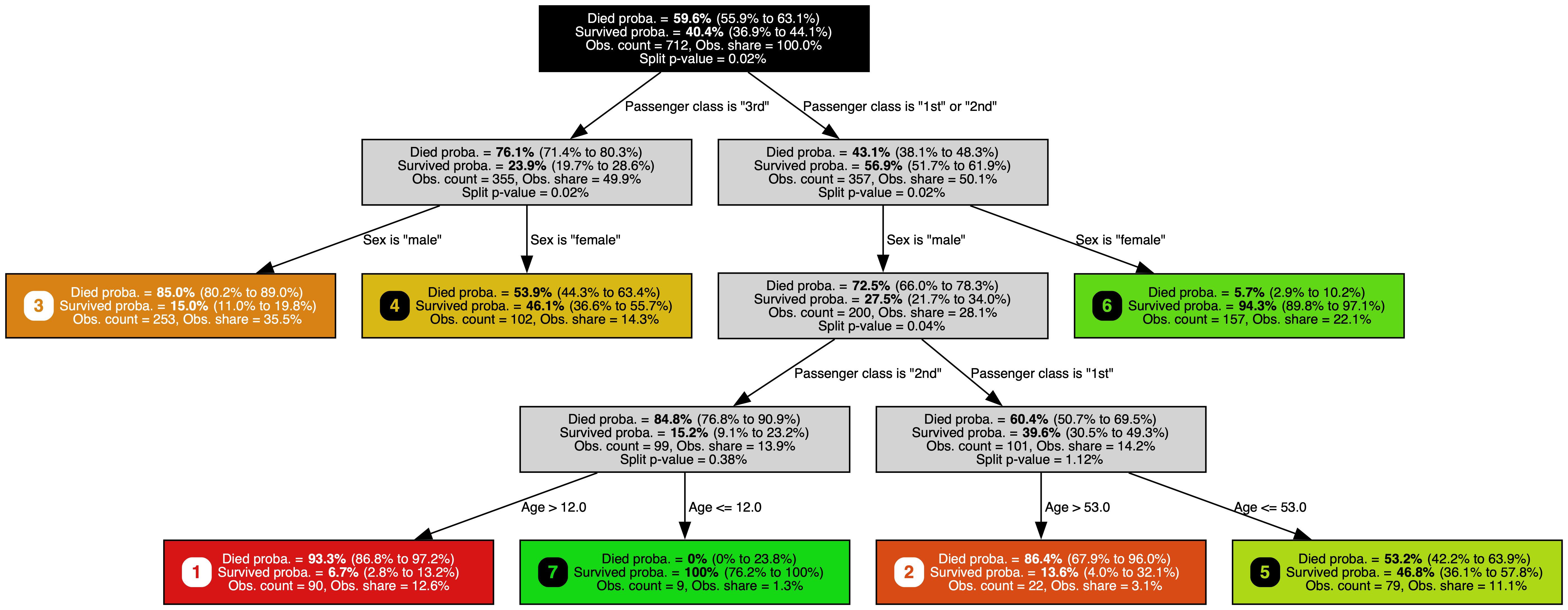
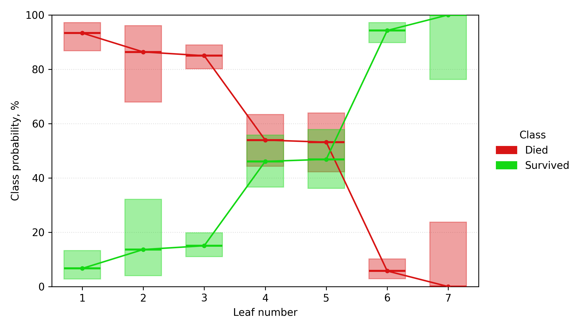
Predicting survival probability with a Jeffreys 95% confidence interval at each node - surfaces passenger class, sex, and age.
tree = sigma.ClassificationTree(random_state=123)
tree.fit(X, y)
print(tree.to_text(precision=1))
tree.to_image("png", "titanic.png", precision=1)
tree.to_image("png", "titanic_response.png", kind="response")
                                                 Died proba.        Survived proba. Obs. count Obs. share Split p-value Leaf index
                                      ---------------------- ---------------------- ---------- ---------- ------------- ----------
All records                           59.6% (55.9% to 63.1%) 40.4% (36.9% to 44.1%)        712     100.0%         0.02%
├── Passenger class is "1st" or "2nd" 43.1% (38.1% to 48.3%) 56.9% (51.7% to 61.9%)        357      50.1%         0.02%
│   ├── Sex is "female"                 5.7% (2.9% to 10.2%) 94.3% (89.8% to 97.1%)        157      22.1%                        6
│   └── Sex is "male"                 72.5% (66.0% to 78.3%) 27.5% (21.7% to 34.0%)        200      28.1%         0.08%
│       ├── Passenger class is "1st"  60.4% (50.7% to 69.5%) 39.6% (30.5% to 49.3%)        101      14.2%         1.02%
│       │   ├── Age <= 53.0           53.2% (42.2% to 63.9%) 46.8% (36.1% to 57.8%)         79      11.1%                        5
│       │   └── Age > 53.0            86.4% (67.9% to 96.0%)  13.6% (4.0% to 32.1%)         22       3.1%                        2
│       └── Passenger class is "2nd"  84.8% (76.8% to 90.9%)  15.2% (9.1% to 23.2%)         99      13.9%         0.62%
│           ├── Age <= 12.0                 0% (0% to 23.8%)   100% (76.2% to 100%)          9       1.3%                        7
│           └── Age > 12.0            93.3% (86.8% to 97.2%)   6.7% (2.8% to 13.2%)         90      12.6%                        1
└── Passenger class is "3rd"          76.1% (71.4% to 80.3%) 23.9% (19.7% to 28.6%)        355      49.9%         0.02%
    ├── Sex is "female"               53.9% (44.3% to 63.4%) 46.1% (36.6% to 55.7%)        102      14.3%                        4
    └── Sex is "male"                 85.0% (80.2% to 89.0%) 15.0% (11.0% to 19.8%)        253      35.5%                        3
 |
 |
4.2. Diabetes (regression)
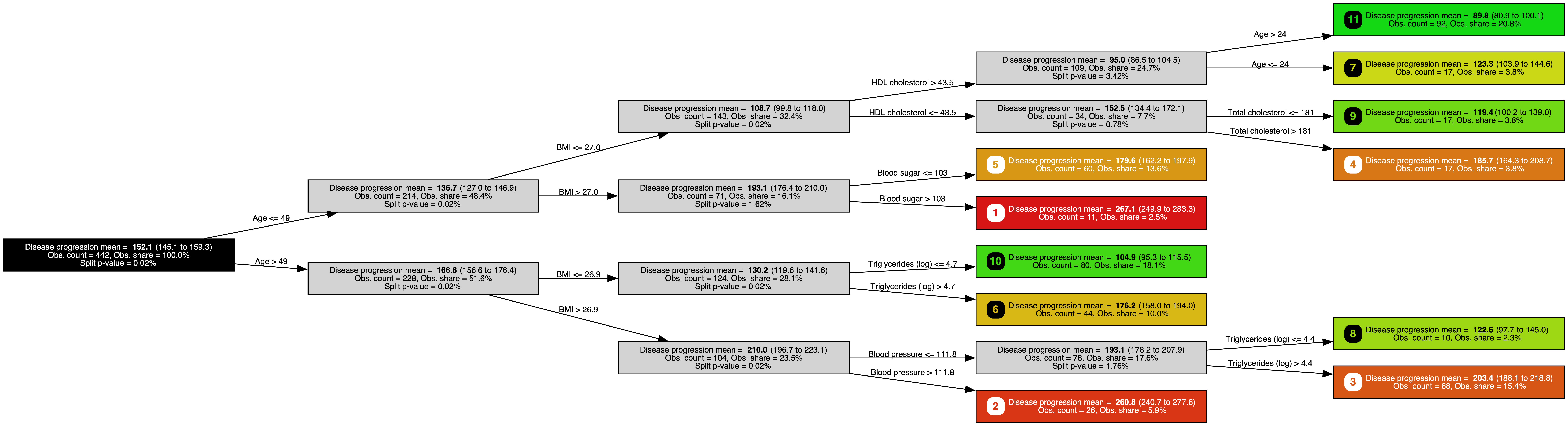
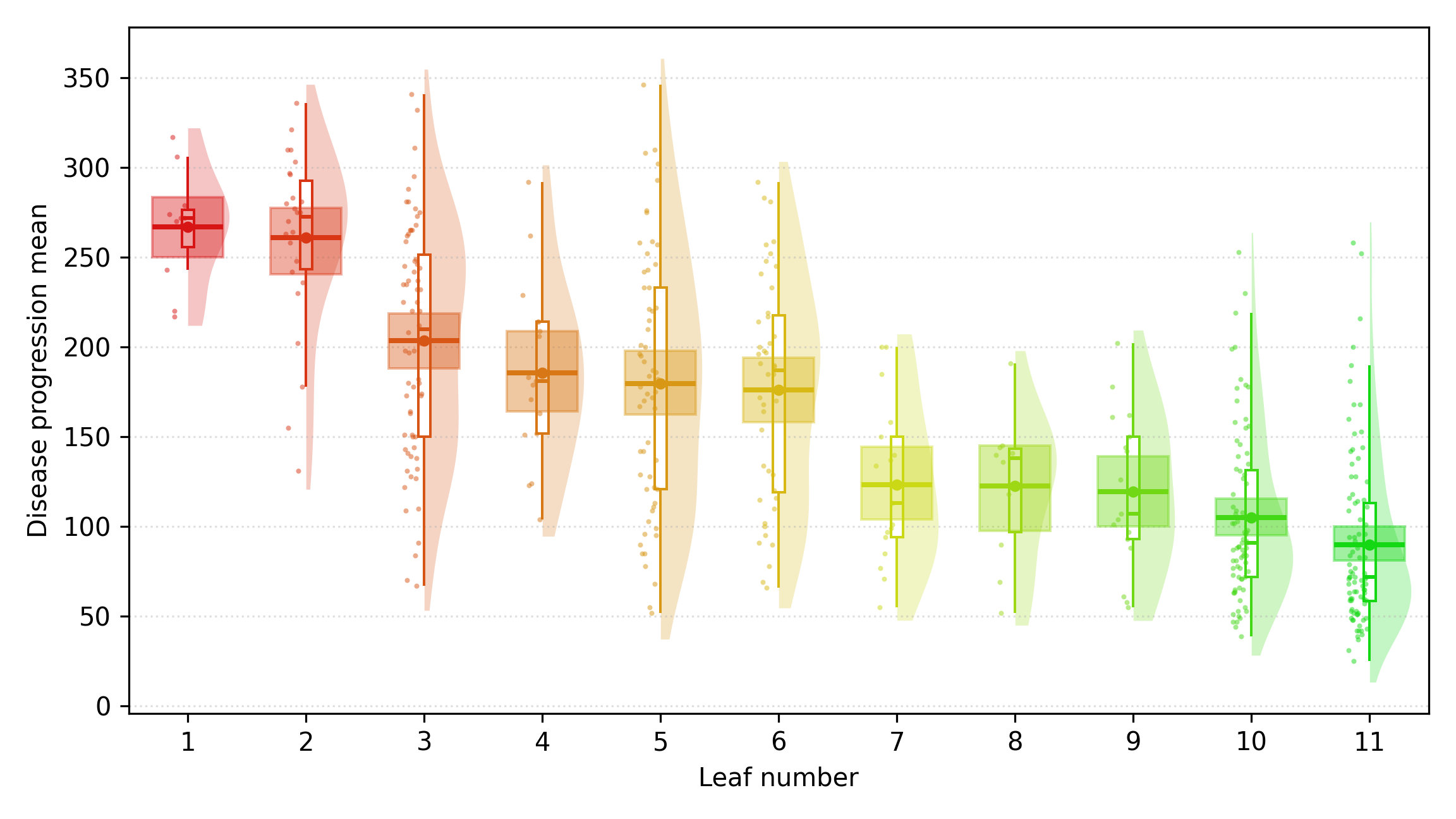
Predicting one-year disease progression with a Bayesian-bootstrap 95%
confidence interval at each node - surfaces BMI, triglycerides, and blood
pressure. BMI splits recursively, so the example calls compact() (see
section 5.5) to fold that chain into one multi-way node.
tree = sigma.RegressionTree(
    test_type="monte_carlo",
    resamples=2000,
    random_state=123,
    reverse_order=True,
)
tree.fit(X, y)
compact_tree = tree.compact()
print(compact_tree.to_text(precision=1))
compact_tree.to_image(
    "png", "diabetes.png", orientation="left-to-right", precision=1
)
compact_tree.to_image("png", "diabetes_response.png", kind="response")
                                       Disease progression mean Obs. count Obs. share Split p-value Leaf index
                                       ------------------------ ---------- ---------- ------------- ----------
All records                              152.1 (145.1 to 159.4)        442     100.0%
├── BMI <= 24.4                           105.0 (97.6 to 112.9)        165      37.3%         0.05%
│   ├── Triglycerides (log) <= 4.6         93.9 (86.7 to 101.4)        123      27.8%                        8
│   └── Triglycerides (log) > 4.6        137.7 (121.6 to 153.6)         42       9.5%                        6
├── 24.4 < BMI <= 27.2                   144.0 (131.5 to 157.1)        112      25.3%         0.05%
│   ├── Total-to-HDL ratio <= 4.8        118.4 (104.3 to 133.9)         65      14.7%         0.05%
│   │   ├── Triglycerides (log) <= 4.8    102.2 (89.5 to 116.4)         53      12.0%                        7
│   │   └── Triglycerides (log) > 4.8    190.0 (162.1 to 217.8)         12       2.7%                        3
│   └── Total-to-HDL ratio > 4.8         179.3 (160.8 to 197.9)         47      10.6%                        4
└── BMI > 27.2                           204.8 (193.8 to 215.4)        165      37.3%         0.05%
    ├── Blood pressure <= 111.8          189.3 (176.8 to 201.6)        124      28.1%         0.05%
    │   ├── Triglycerides (log) <= 5.1   171.1 (156.4 to 186.8)         80      18.1%                        5
    │   └── Triglycerides (log) > 5.1    222.5 (205.0 to 238.2)         44      10.0%                        2
    └── Blood pressure > 111.8           251.4 (235.1 to 265.8)         41       9.3%                        1
 |
 |
4.3. GBSG-2 breast cancer (survival)
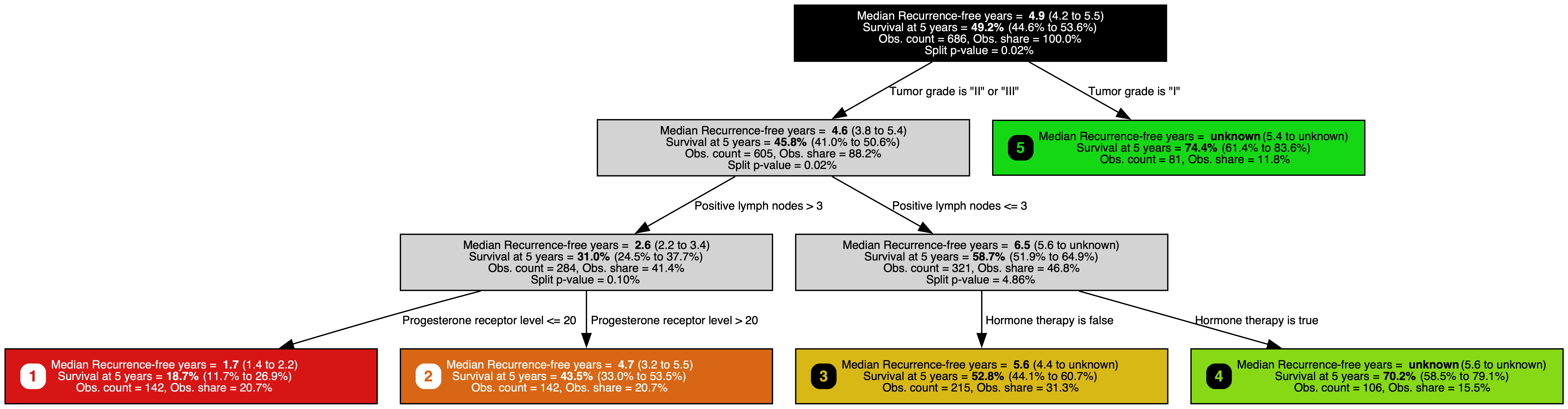
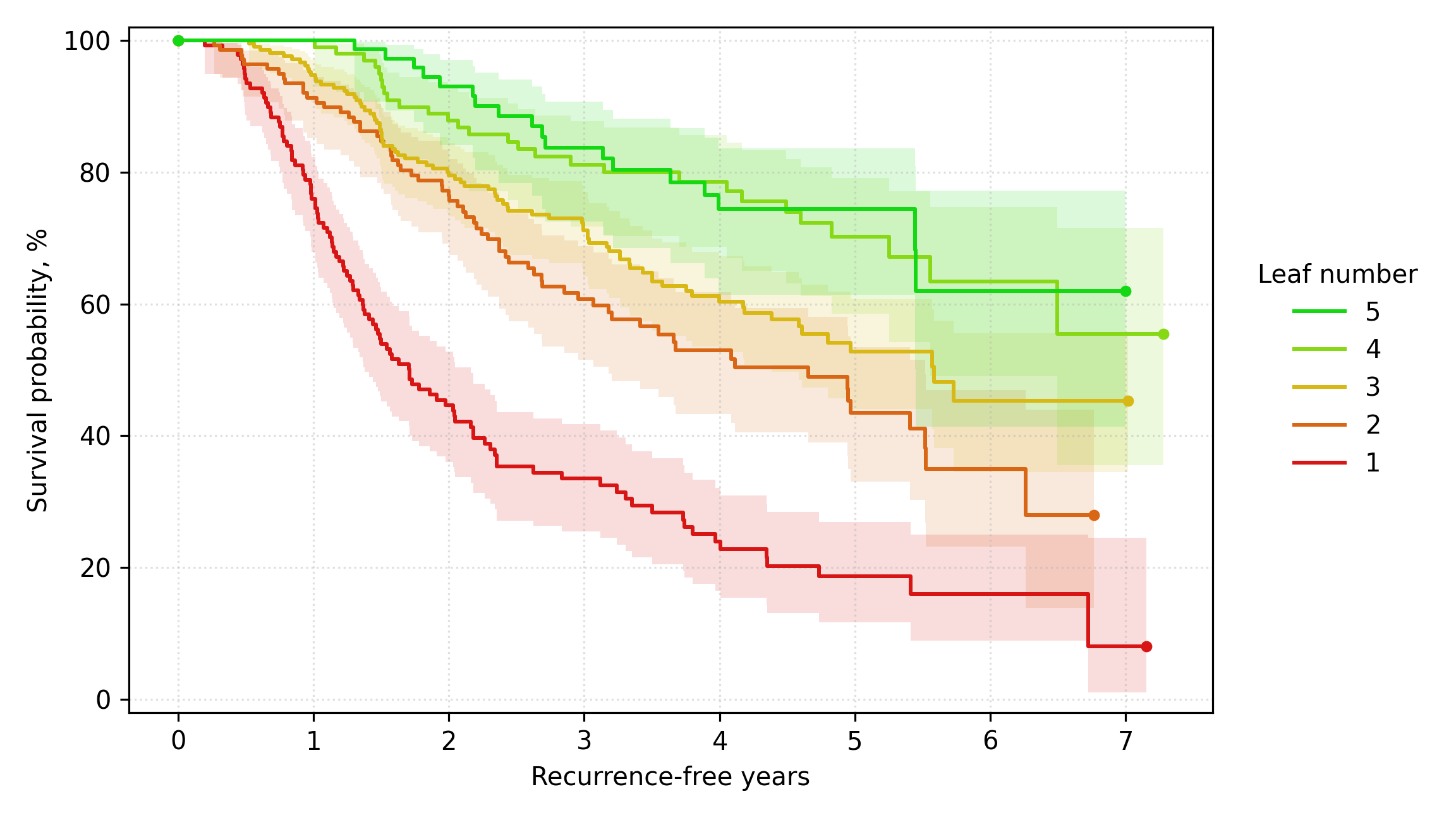
Predicting recurrence-free years with a Brookmeyer-Crowley 95% confidence interval at each node - splits on positive lymph nodes, hormone therapy, and progesterone receptor level.
tree = sigma.SurvivalTree(
    random_state=123,
    metrics=("median", ("survival", 5.0, "years")),
)
tree.fit(X, y)
print(tree.to_text(precision=1))
tree.to_image("png", "breast_cancer.png", precision=1)
tree.to_image("png", "breast_cancer_response.png", kind="response")
                                              Median Recurrence-free years    Survival at 5 years Obs. count Obs. share Split p-value Leaf index
                                              ---------------------------- ---------------------- ---------- ---------- ------------- ----------
All records                                               4.9 (4.2 to 5.5) 49.2% (44.6% to 53.6%)        686     100.0%         0.02%
├── Tumor size <= 19                              unknown (5.4 to unknown) 65.6% (55.4% to 73.9%)        135      19.7%         0.04%
│   ├── Positive lymph nodes <= 2                 unknown (unknown bounds) 80.7% (68.2% to 88.7%)         77      11.2%                        7
│   └── Positive lymph nodes > 2                          4.7 (2.6 to 5.5) 44.7% (29.2% to 59.1%)         58       8.5%         3.52%
│       ├── Age > 41                                  5.4 (3.5 to unknown) 54.6% (36.2% to 69.8%)         49       7.1%                        5
│       └── Age <= 41                                     1.3 (0.7 to 3.2)          0% (0% to 0%)          9       1.3%                        1
└── Tumor size > 19                                       4.3 (3.7 to 5.0) 44.9% (39.7% to 49.9%)        551      80.3%         0.02%
    ├── Positive lymph nodes <= 4                     5.7 (4.8 to unknown) 54.7% (47.7% to 61.0%)        332      48.4%         1.10%
    │   ├── Hormone therapy is true               unknown (5.6 to unknown) 67.7% (56.3% to 76.7%)        114      16.6%                        6
    │   └── Hormone therapy is false                  4.8 (3.9 to unknown) 47.1% (38.3% to 55.4%)        218      31.8%                        4
    └── Positive lymph nodes > 4                          2.4 (2.0 to 3.1) 29.9% (22.6% to 37.5%)        219      31.9%         0.10%
        ├── Progesterone receptor level > 24              4.1 (2.7 to 5.5) 43.8% (31.4% to 55.4%)        107      15.6%                        3
        └── Progesterone receptor level <= 24             1.7 (1.4 to 2.2) 17.3% (10.0% to 26.3%)        112      16.3%                        2
 |
 |
4.4. Sushi (ranking)
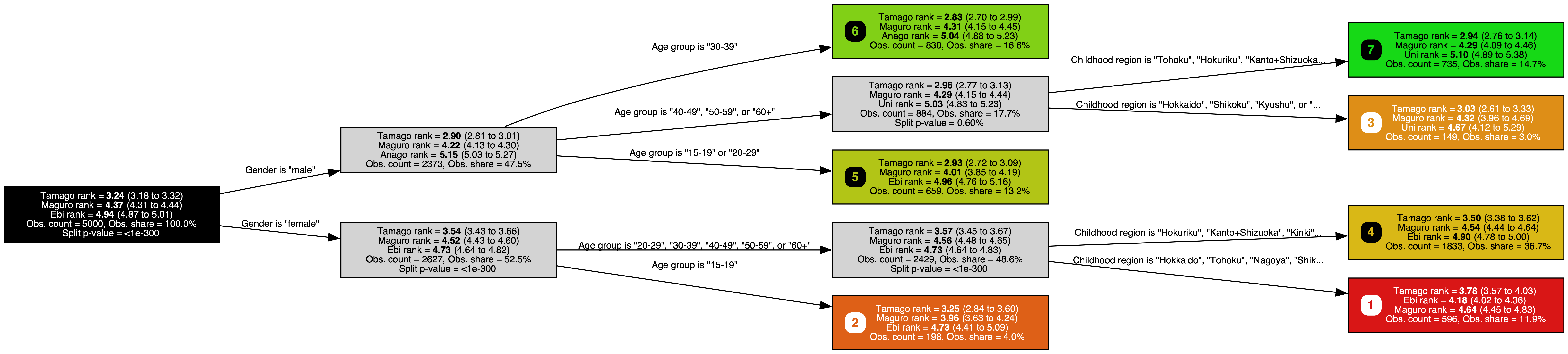
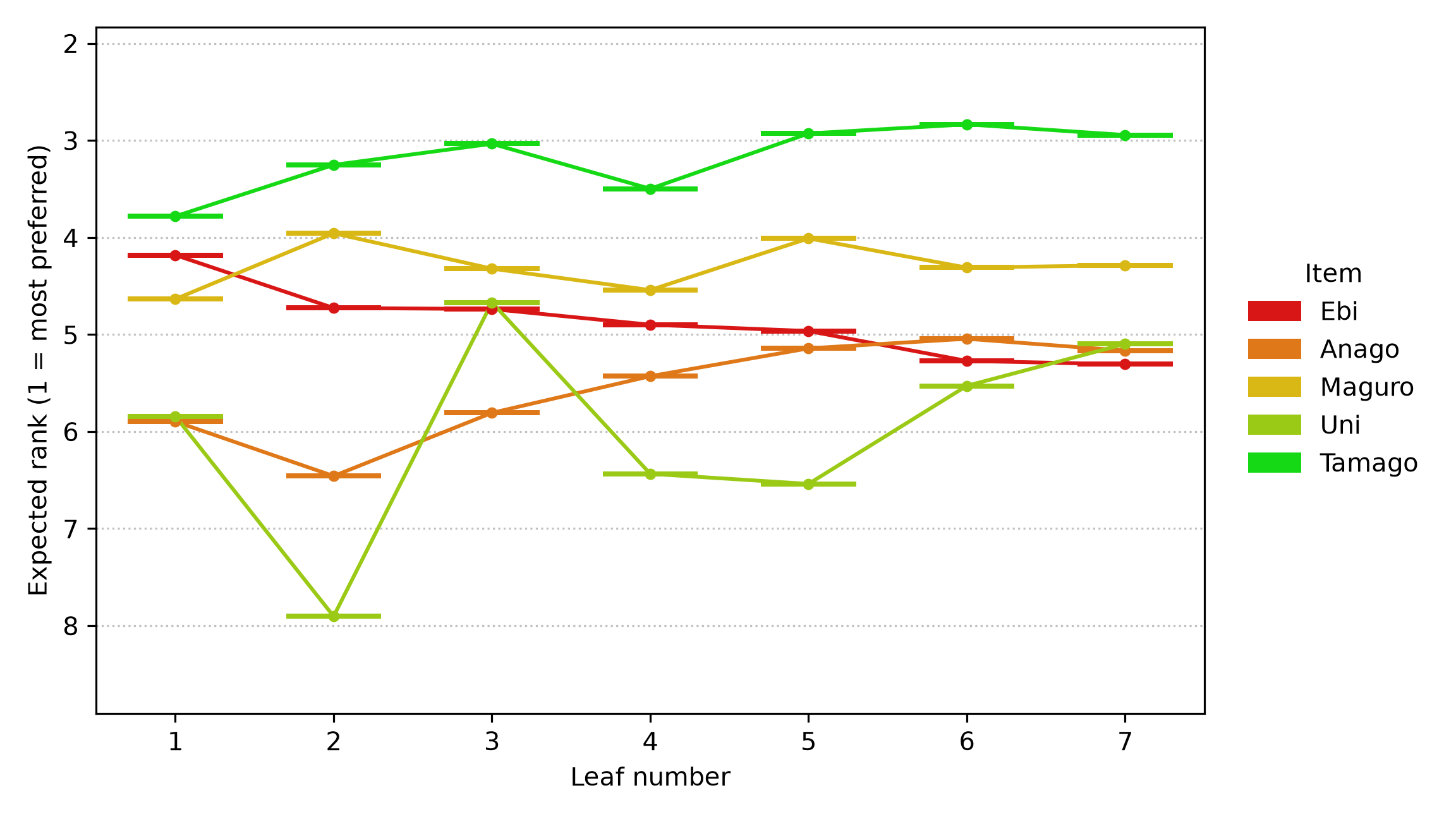
Predicting per-item Plackett-Luce expected rank with a Bayesian-bootstrap
95% confidence interval at each node - surfaces sex and age group as the
strongest demographic drivers of sushi preference among 5000 Japanese
respondents ranking ten classic sushi. Age group splits recursively on the
male side, so the example calls compact() (see section 5.5) to fold that
chain into one multi-way node.
tree = sigma.RankingTree(
    pca_components=10,
    random_state=123,
    max_depth=3,
)
tree.fit(X, rankings)
compact_tree = tree.compact()
print(compact_tree.to_text(precision=2))
compact_tree.to_image(
    "png", "sushi.png", orientation="left-to-right", precision=2
)
compact_tree.to_image("png", "sushi_response.png", kind="response")
                                                                                                                              Ebi rank          Anago rank         Maguro rank            Uni rank         Tamago rank Obs. count Obs. share Split p-value Leaf index
                                                                                                                   ------------------- ------------------- ------------------- ------------------- ------------------- ---------- ---------- ------------- ----------
All records                                                                                                        4.94 (4.86 to 5.01) 5.39 (5.32 to 5.46) 4.37 (4.31 to 4.43) 6.07 (5.98 to 6.16) 3.24 (3.15 to 3.31)       5000     100.0%       <1e-300
├── Gender is "male"                                                                                               5.16 (5.05 to 5.25) 5.15 (5.06 to 5.28) 4.22 (4.11 to 4.33) 5.66 (5.50 to 5.77) 2.90 (2.82 to 3.01)       2373      47.5%
│   ├── Age group is "30-39"                                                                                       5.27 (5.14 to 5.43) 5.04 (4.83 to 5.23) 4.31 (4.18 to 4.45) 5.53 (5.30 to 5.75) 2.83 (2.71 to 2.99)        830      16.6%                        6
│   ├── Age group is "40-49", "50-59", or "60+"                                                                    5.21 (5.04 to 5.39) 5.28 (5.12 to 5.45) 4.29 (4.15 to 4.44) 5.03 (4.80 to 5.23) 2.96 (2.81 to 3.13)        884      17.7%         0.60%
│   │   ├── Childhood region is "Tohoku", "Hokuriku", "Kanto+Shizuoka", "Nagoya", "Kinki", "Chugoku", or "Okinawa" 5.31 (5.13 to 5.50) 5.17 (4.97 to 5.34) 4.29 (4.14 to 4.43) 5.10 (4.88 to 5.33) 2.94 (2.76 to 3.15)        735      14.7%                        7
│   │   └── Childhood region is "Hokkaido", "Shikoku", "Kyushu", or "abroad"                                       4.74 (4.36 to 5.13) 5.81 (5.37 to 6.23) 4.32 (3.98 to 4.66) 4.67 (4.23 to 5.19) 3.03 (2.66 to 3.35)        149       3.0%                        3
│   └── Age group is "15-19" or "20-29"                                                                            4.96 (4.78 to 5.14) 5.14 (4.95 to 5.34) 4.01 (3.84 to 4.17) 6.54 (6.30 to 6.73) 2.93 (2.73 to 3.15)        659      13.2%                        5
└── Gender is "female"                                                                                             4.73 (4.64 to 4.82) 5.62 (5.53 to 5.72) 4.52 (4.43 to 4.59) 6.44 (6.32 to 6.55) 3.54 (3.43 to 3.66)       2627      52.5%       <1e-300
    ├── Age group is "20-29", "30-39", "40-49", "50-59", or "60+"                                                  4.73 (4.63 to 4.82) 5.55 (5.44 to 5.66) 4.56 (4.48 to 4.65) 6.30 (6.13 to 6.41) 3.57 (3.46 to 3.68)       2429      48.6%       <1e-300
    │   ├── Childhood region is "Hokuriku", "Kanto+Shizuoka", "Kinki", "Chugoku", "Kyushu", or "abroad"            4.90 (4.78 to 5.01) 5.43 (5.28 to 5.57) 4.54 (4.46 to 4.63) 6.44 (6.31 to 6.59) 3.50 (3.38 to 3.62)       1833      36.7%                        4
    │   └── Childhood region is "Hokkaido", "Tohoku", "Nagoya", "Shikoku", or "Okinawa"                            4.18 (4.02 to 4.38) 5.90 (5.70 to 6.12) 4.64 (4.47 to 4.82) 5.84 (5.55 to 6.13) 3.78 (3.61 to 3.99)        596      11.9%                        1
    └── Age group is "15-19"                                                                                       4.73 (4.37 to 5.11) 6.46 (6.08 to 6.79) 3.96 (3.68 to 4.30) 7.90 (7.60 to 8.25) 3.25 (2.88 to 3.64)        198       4.0%                        2
 |
 |
5. Advanced usage
5.1. Controlling tree depth and node size
alpha is the principal knob: it sets the significance threshold for
every split test, so lowering it produces a terser, more statistically
conservative tree, and raising it produces a richer, more exploratory
one. min_splits, min_buckets, and max_depth are secondary safety
bounds.
tree = sigma.ClassificationTree(
    max_depth=4,            # maximum tree depth (None = unlimited)
)
5.2. Fitting with sample weights
Sample weights let you model variable exposures - per-row
time-at-risk, insurance policy-years, or frequency weights for
pre-aggregated rows. A weight of k is equivalent to observing the
sample k times for regression, classification, and ranking; for
survival the weights enter the log-rank risk sets, so the exact
row-repetition equivalence does not hold.
import numpy
from sigma import RegressionTree

n = 200
X = numpy.random.randn(n, 2)
claim_amount = numpy.where(X[:, 0] > 0, 1500.0, 300.0) + 100 * numpy.random.randn(n)
exposure_years = numpy.random.uniform(0.1, 2.0, size=n)

tree = RegressionTree()
tree.fit(X, claim_amount, sample_weight=exposure_years)
predictions = tree.predict(X)
5.3. Visualizing the tree
Install the optional visualization extra and the Graphviz system
binary (brew install graphviz on macOS):
pip install ars-sigma[viz]
Then render to PNG, PDF, SVG, or GIF:
tree.to_image("png", "tree.png", feature_names=["feature_1", "feature_2"], response_name="y")
All four formats are produced directly by the Graphviz binary, with no
additional system library. See to_image and export_graphviz for the
full set of display options.
5.4. Exporting the tree as a SQL CASE expression
to_sql (and the module-level sigma.export_sql) emits a single SQL
CASE expression that reproduces tree.predict row-by-row in any
SQL-92/SQL-99 engine, with no extra dependencies:
sql_expression = tree.to_sql()
print(sql_expression)
# SELECT id, (<sql_expression>) AS prediction FROM points;
CASE
    WHEN "Passenger class" IN ('1st', '2nd') THEN
        CASE
            WHEN "Sex" = 'female' THEN
                0.9426751592356688 -- Leaf 6
            WHEN "Sex" = 'male' THEN
                CASE
                    WHEN "Passenger class" = '1st' THEN
                        CASE
                            WHEN "Age" <= 53.0 THEN
                                0.46835443037974683 -- Leaf 5
                            WHEN "Age" > 53.0 THEN
                                0.13636363636363635 -- Leaf 2
                            ELSE NULL
                        END
                    WHEN "Passenger class" = '2nd' THEN
                        CASE
                            WHEN "Age" <= 12.0 THEN
                                1.0 -- Leaf 7
                            WHEN "Age" > 12.0 THEN
                                0.06666666666666667 -- Leaf 1
                            ELSE NULL
                        END
                    ELSE 0.275
                END
            ELSE 0.5686274509803921
        END
    WHEN "Passenger class" = '3rd' THEN
        CASE
            WHEN "Sex" = 'female' THEN
                0.46078431372549017 -- Leaf 4
            WHEN "Sex" = 'male' THEN
                0.15019762845849802 -- Leaf 3
            ELSE 0.23943661971830985
        END
    ELSE 0.4044943820224719
END
For ClassificationTree, pass target_class= to pick which class
probability the expression should emit. Categorical values not seen at
fit time evaluate to the holding node's prediction, mirroring
tree.predict. NULL numerical or boolean inputs fall through to
ELSE NULL; wrap in COALESCE(..., default) to substitute a fallback
value.
5.5. Collapsing recursive splits with compact()
When the same feature is split over several consecutive levels, a binary
tree repeats that feature down a chain. compact() returns a new tree in
which each such chain is collapsed into a single multi-way node, with one
branch per resulting interval (numeric features) or category subset
(categorical features):
compact_tree = tree.compact()
print(compact_tree.to_text())
The compacted tree predicts identically to the original and renders
through the same to_text, to_image, and to_sql methods. A merged
node spans several original splits, so it reports no single split
p-value. For example, a chain of consecutive splits on Age
├── Age <= 30
└── Age > 30
    ├── Age <= 50
    └── Age > 50
collapses into one node carrying three interval branches:
├── Age <= 30
├── 30 < Age <= 50
└── Age > 50
The original tree is left unchanged; compact() produces an independent
copy whose node ids are renumbered to match its smaller shape.
6. Parameters
The table below is a quick reference; each parameter has a dedicated subsection further down with defaults, alternatives, and guidance on when to choose each option.
| Parameter | Description |
|---|---|
correlation |
Rank-transform inputs (robust) or use raw values (classical) |
test_stat |
How the multivariate score is aggregated into a scalar test statistic |
test_type |
Multiplicity adjustment applied across covariates |
alpha |
Significance level for the stopping rule |
min_splits |
Minimum sum of weights required to attempt a split |
min_buckets |
Minimum sum of weights in each child node |
max_depth |
Maximum tree depth |
categorical_features |
Which feature columns are categorical |
ci_method (classification tree) |
Confidence interval method for per-class proportions |
ci_method (regression tree) |
Confidence interval method for node mean predictions |
ci_method (ranking tree) |
Confidence interval method for per-item leaf PL-MLE expected-rank predictions |
ci_method (survival tree) |
Confidence interval method for the median survival time |
ci_coverage |
Coverage level for node-prediction confidence intervals |
ci_replicates (ranking tree) |
RankingTree bootstrap replicates for the resampling CI methods |
npseudo |
Turner ghost-item pseudo-comparison weight for the per-node PL fit |
pl_max_iter |
Maximum Hunter MM iterations per node's Plackett-Luce fit |
pl_tolerance |
Convergence tolerance on log-worth for the Hunter MM iteration |
pca_components (ranking tree) |
RankingTree principal components of the per-node log-rank matrix |
item_names (ranking tree) |
RankingTree display labels for the ranked items |
metrics (survival tree) |
SurvivalTree per-node metrics to compute and render |
response_sample_size |
RegressionTree response-sample cap for the response plot |
transmuter |
Per-node data transform with post-hoc split validation |
resamples |
Number of permutations for test_type="monte_carlo" |
decorator |
Per-node decoration callable rendered by to_text / to_image |
reverse_order |
Reverse the canonical leaf display order across all renderings |
random_state |
RNG seed for permutation resampling, bootstrap CI methods, and plot jitter |
6.1. correlation
Default: "rank" (SurvivalTree defaults to "normal", matching
partykit's survival behavior).
Score function for the test statistic.
"normal"uses raw values, recovering the original Pearson-like behavior from Hothorn et al. (2006). Choose this when the response is well-behaved (approximately Gaussian, no heavy outliers) and you want the slight power gain on truly linear associations."rank"(default) rank-transforms continuous covariates and, for regression, the response before computing the statistic, yielding a Spearman-like nonparametric test. Robust to outliers and heavy tails. The safe choice for arbitrary real-world data.
6.2. test_stat
Default: "quadratic".
How the multivariate score is aggregated into a scalar test statistic.
"maximum"is a maximum-type statistic that concentrates power on alternatives where one component dominates. Choose this when you expect a single-direction effect (e.g., a binary classification where only one class differs from the rest)."quadratic"(default) is an omnibus chi-squared form with good power across general alternatives. Choose this when you have no prior on the direction of association, or when the response is multivariate (multi-class classification with many classes).
6.3. test_type
Default: "sidak".
Multiplicity adjustment applied across the $m$ candidate covariates (indexed by $j$), transforming each raw p-value $P_j$ before the stopping rule fires.
"bonferroni"is the closed-form $\min(m P_j, 1)$. The simplest and best-known correction, strictly more conservative than Sidak under independence; prefer"sidak"unless matching an external reference."monte_carlo"is the Westfall-Young min-P resampling procedure. More powerful than Sidak when covariates are correlated, at the cost of $B \cdot m$ extra statistic evaluations per node, where $B$ is the number of response permutations (controlled byresamples). Choose when covariates are highly collinear and you can afford the resampling budget; requires a positiveresamples."sidak"(default) is the closed-form $1 - (1 - P_j)^m$. Powerful under independence or positive dependence of test statistics. The recommended default.
6.4. alpha
Default: 0.05.
Significance level for the stopping rule. Recursion stops at a node when $\min_j(\text{adjusted } P_j) > \alpha$.
The default 0.05 is a good choice for simple, exploratory analysis.
For trees fitted on very large datasets, or on correlated records
where the independence assumption is partially broken, tighten
alpha by one or two orders of magnitude (0.005 or 0.0005) to
keep the tree compact. For models aiming at higher predictive
accuracy (closer to a full-fledged machine learning model), loosen
alpha to between 0.10 and 0.25. Tune in concert with
max_depth, min_splits, and min_buckets.
6.5. min_splits
Default: 20.
Minimum sum of weights required to attempt a split. Nodes whose weight sum falls below this become leaves regardless of p-values. Increase to enforce statistical reliability of node-level estimates on smaller subsets, decrease to allow finer partitioning.
6.6. min_buckets
Default: 7.
Minimum sum of weights in each child node. Splits that would produce a
child smaller than this are rejected. Together with min_splits,
controls the smallest leaf permitted; raise both for noisier data.
6.7. max_depth
Default: None (no limit).
Maximum tree depth. Set to a small integer for shallow, easily interpreted
trees. Leave None to let the p-value stopping rule fully control depth.
6.8. categorical_features
Default: None (all numeric).
List of feature columns to treat as categorical. Entries may be
column-name strings (resolved against the DataFrame columns at fit
time, i.e. feature_names_in_) or integer column indices; mixing the
two forms is allowed. Letting $K$ denote the number of levels in a
categorical feature, Sigma uses exhaustive split enumeration for
$K \le 10$ and an ordered-merge heuristic for $K > 10$ (see the
Algorithm section).
6.9. ci_method (RegressionTree only)
Default: "bayesian_bootstrap".
Method for the confidence interval on each node's mean prediction. In the descriptions below, $y$ denotes the per-row response, $n$ the sample size at the node, and $n_{\text{eff}}$ the Kish effective sample size at the node.
"bayesian_bootstrap"(default) uses Dirichlet resampling of the weighted mean. Nonparametric: makes no assumption on the response distribution. The safe choice for arbitrary regression targets, but less powerful than a method tailored to the response's actual distribution."bca"is the bias-corrected and accelerated bootstrap interval (Efron, 1987): resample $10{,}000$ times from the empirical distribution, then read percentiles corrected for median bias ($z_0$) and skewness ($a$, computed via jackknife). Nonparametric and second-order accurate ($O(1/n)$ coverage error); transformation-respecting. Choose for the frequentist counterpart of"bayesian_bootstrap"when an external benchmark specifies a frequentist confidence interval. Non-deterministic across calls."beta"is a Clopper-Pearson-style Beta interval for proportional responses in $[0, 1]$. Choose when $y$ is naturally a rate or proportion (conversion rate, click-through rate)."exponential"is the exact chi-squared interval for an Exponential mean (Gamma with shape $= 1$); requires $y \ge 0$. Choose when responses are non-negative waiting times or lifetimes that follow an exponential distribution."gamma"is the exact chi-squared interval for a Gamma mean using a method-of-moments shape estimate; requires $y \ge 0$. Choose for non-negative right-skewed responses (insurance claims, incomes, durations)."log_normal"is Cox's interval for the arithmetic mean of a log-normal response; requires $y > 0$. Centered on the log-normal MLE of the mean, not the sample mean. Choose when $\log y$ is approximately normal (financial returns, biological measurements)."log_normal_gci"is the generalized confidence interval (Krishnamoorthy & Mathew, 2003) for the arithmetic mean of a log-normal response; requires $y > 0$. Like"log_normal"but built via Monte Carlo from a generalized pivot, giving asymmetric bounds. Choose when $n_{\text{eff}}$ is very small with large $\log y$ variance, where Cox's symmetric Wald form begins to lose calibration. Non-deterministic across calls."normal"is a Wald-style interval $\bar{Y} \pm z \cdot \text{SE}$ ($\bar{Y}$ the node weighted mean of $y$, $z$ a standard normal quantile, $\text{SE}$ the standard error) with the Kish effective sample size. Tight and cheap. Choose when the central limit theorem applies comfortably ($n_{\text{eff}}$ well above 30, finite response variance)."poisson"is the exact Garwood chi-squared interval for a Poisson mean rate; requires $y \ge 0$. The conservative choice with guaranteed coverage (Patil & Kulkarni, 2012). Choose for count responses generated by an approximately Poisson process when guaranteed coverage matters more than tightness."poisson_jeffreys"is the equal-tailed Jeffreys interval for a Poisson mean rate; requires $y \ge 0$. Shorter than"poisson"at moderate rates (Patil & Kulkarni, 2012). Choose for count responses at moderate rates when you do not require Garwood's guaranteed coverage."student_t"has the same form as"normal"but uses a Student-t quantile with $n_{\text{eff}} - 1$ degrees of freedom. Wider than"normal"for small effective sample sizes. Choose when $n_{\text{eff}}$ is borderline and small-sample coverage matters.
6.10. ci_method (ClassificationTree only)
Default: "jeffreys".
Method for the per-class confidence intervals on node class proportions. In the descriptions below, $n$ denotes the node sample size and $z$ a standard normal quantile.
"agresti_coull"is the adjusted Wald interval: Wald applied after adding $z^2/2$ pseudo-successes and $z^2/2$ pseudo-failures. Slightly wider and more conservative than"wilson"at small sample sizes; statistically equivalent to"wilson"and"jeffreys"for $n > 40$ per Brown-Cai-DasGupta (2001). Choose when matching an external reference that specifies Agresti-Coull."clopper_pearson"is the exact Beta interval. Has the absolute coverage guarantee ($\ge$ci_coveragefor every true proportion), but is conservative: intervals are wider than they need to be on average. Choose when guaranteed coverage matters more than tightness (regulatory or safety contexts)."jeffreys"(default) is a Bayesian interval from the Beta posterior with the Jeffreys non-informative prior $\mathrm{Beta}(0.5, 0.5)$. Neither systematically conservative nor systematically aggressive on average. Recommended for general use."mid_p_exact"is the mid-p variant of Clopper-Pearson. Strictly narrower than"clopper_pearson"while keeping an exact-tail rationale, with average coverage close to nominal. Choose when Clopper-Pearson's conservatism feels too wasteful but an exact-tail method is still desired."wilson"is the closed-form Wilson score interval, clipped to $[0, 1]$. Cheapest to compute and accurate at moderate sample sizes; coverage degrades near 0 and 1. Choose when you need vectorized speed and class proportions are not extreme."wilson_cc"is the Wilson score interval with Newcombe's continuity correction. Slightly wider than"wilson", restoring lower-tail coverage at small sample sizes. Choose when the node total weight $w_{\text{total}}$ is small and plain Wilson under-covers.
6.11. ci_method (RankingTree only)
Default: "bayesian_bootstrap".
Method for the per-item confidence intervals on each node's Plackett-Luce
expected-rank vector. All four methods target the per-item expected rank;
scalar-mean CI methods ("normal", "student_t") and the seven
distribution-specific methods of RegressionTree ("beta",
"exponential", "gamma", "log_normal", "log_normal_gci",
"poisson", "poisson_jeffreys") are rejected at construction time
because PL expected rank is a non-linear functional of a joint MLE rather
than a scalar sample mean. The resampling methods draw ci_replicates
replicates each.
"bayesian_bootstrap"(default) draws Dirichlet weights for the active rows and refits the PL MLE on each replicate. Nonparametric; the safe choice."bca"is the bias-corrected and accelerated bootstrap (Efron, 1987) applied to row-resampled PL refits, with the acceleration term computed from a leave-one-out jackknife of PL refits. Slower than"bayesian_bootstrap"; non-deterministic across calls."wald"is a closed-form asymptotic interval from the observed PL Fisher information, propagated onto each per-item expected rank. The cheapest method and the only deterministic one;ci_replicatesis ignored. Choose when speed matters and node sample sizes are large."gaussian_multiplier"is a multiplier-CLT bootstrap forming percentile intervals from Gaussian-weighted score perturbations linearised through the Fisher information. Non-deterministic across calls.
6.12. ci_coverage
Default: 0.95.
Coverage level for node-prediction confidence intervals. Set to None
to skip CI computation entirely (the proper way to fully avoid the
per-node ci_method cost). Common alternatives: 0.90 (less
conservative), 0.99 (more conservative). For survival trees, also
controls the confidence band drawn behind each Kaplan-Meier curve in
the response plot; for ranking trees, it sets the per-item whisker
width in the expected-rank response plot.
6.13. transmuter
Default: None.
Optional callable that transforms node-level data before predictions
and confidence intervals are computed, with post-hoc split validation.
Signature: (X, y, sample_weight) -> (y', sample_weight'), or
(X, y, sample_weight, side_data) -> (y', sample_weight') when
side_data is passed to fit. After each candidate split, both
child subsets are independently transmuted and a significance test is
run on the transmuted data; if the p-value exceeds alpha the split
is rejected and the node becomes a leaf. Use cases: survival outcomes
(Kaplan-Meier-style transformation), rate normalization (impressions
to click-through rate), de-noising heavy-tailed responses. RankingTree
does not support a transmuter and rejects one at construction time.
6.14. resamples
Default: None.
Number of permutations $B$ for test_type="monte_carlo". Required and
must be a positive integer when monte_carlo is selected; ignored
otherwise. Typical choices: 1000 for day-to-day production, 10000
for paper-grade reproducible adjusted p-values.
6.15. decorator
Default: None.
Optional callable invoked once per node after the tree is built.
Signature: (X_active, y_active, w_active, side_data_active) -> decoration where decoration is any object (or None). The returned
object is stored on the node as node.decoration and rendered by
to_text and to_image. Use cases: per-node metric (RMSE,
classification accuracy), business labels (segment names), diagnostic
statistics.
6.16. random_state
Default: None.
Seed for all stochastic operations in the estimator. Pass an integer
for reproducibility; None uses an unpredictable seed. Controls:
- min-P permutation resampling under
test_type="monte_carlo"; - the bootstrap-family CI methods of
RegressionTree(bayesian_bootstrap,bca,log_normal_gci); - the resampling CI methods of
RankingTree(bayesian_bootstrap,bca,gaussian_multiplier) applied K times per node - once per item; - the jitter of
to_image(kind="response")raincloud plots (RegressionTreeonly; combined with the leaf index so each leaf receives a distinct pattern).
6.17. ci_method (SurvivalTree only)
Default: "brookmeyer_crowley".
Method for the confidence interval on each node's median survival time.
"brookmeyer_crowley" (default) is the Brookmeyer-Crowley interval and
the only supported option.
6.18. ci_replicates (RankingTree only)
Default: 200.
Number of bootstrap replicates drawn by the resampling ci_method
choices ("bayesian_bootstrap", "bca", "gaussian_multiplier").
Ignored when ci_method="wald". Raise for smoother interval estimates
at higher cost.
6.19. npseudo (RankingTree only)
Default: 0.5.
Weight of the Turner ghost-item pseudo-comparisons added to each item during the per-node Plackett-Luce fit. Must be strictly positive. The default follows Turner et al. (2020); raise it to regularize nodes with few or sparsely overlapping rankings.
6.20. pl_max_iter (RankingTree only)
Default: 100.
Maximum number of Hunter MM iterations for each node's Plackett-Luce fit. Must be a positive integer. Raise it if the fit fails to converge on large catalogues.
6.21. pl_tolerance (RankingTree only)
Default: 1e-6.
Convergence tolerance on the largest change in log-worth between successive MM iterations. Must be strictly positive. Lower it for tighter fits at higher cost.
6.22. pca_components (RankingTree only)
Default: 10.
Number of principal components of the per-node log-rank matrix used as the influence function for the split tests. Must be at least 1. When it is at least the catalogue size, the projection covers the full response space; lower it to denoise high-dimensional rankings.
6.23. item_names (RankingTree only)
Default: None.
Display labels for the ranked items, one per item. When None and the
rankings are a NumPy array, integer indices 0..n_items-1 are used; when
the rankings are a pandas DataFrame, its column names take precedence
over this argument.
6.24. metrics (SurvivalTree only)
Default: ("median",).
Sequence of per-node survival metrics to compute and render. Each entry
is either a string for parameter-free metrics ("median",
"risk_score") or a tuple (kind, value, unit) for parametrized metrics
("survival", "rmst"), where value is in the response's time units
and unit is the trailing label token. For example,
("survival", 5.0, "years") renders as "Survival at 5 years". Metrics
render in the given order; the first drives the leaf ordering and the
value returned by predict. The default predicts the median survival
time.
6.25. response_sample_size (RegressionTree only)
Default: 1000.
Maximum number of response values stored on each leaf for the
response-distribution overlay in to_image(kind="response"). Must be a
non-negative integer. Set to 0 to store none, yielding smaller fitted
trees with no raincloud overlay.
6.26. reverse_order
Default: False.
When True, reverses the canonical leaf ordering used by leaves_,
to_text, to_image, and to_sql (the per-task sort described in
section 8). Use it to flip the reading direction, for example to list
the best-prognosis leaf first.
7. Algorithm
The algorithm builds a decision tree using statistical hypothesis testing for unbiased variable selection. Unlike CART, which selects variables by maximizing an impurity criterion (and is therefore biased toward variables with many possible splits), conditional inference trees use permutation-based p-values to decouple variable selection from split search.
The framework is generic: the only difference between the four task families is the influence function $h$ applied to the response $Y_i$ of observation $i$. For classification with $J$ classes, $h(Y_i) = e_J(Y_i)$ (one-hot encoding of the class label). For regression, $h(Y_i) = Y_i$ (identity). For survival, $h(Y_i)$ is the log-rank score (a scalar centred Savage score). For ranking, the ranks-in-cell $Y_i$ is imputed at unranked items with the per-row tail mean, log-transformed via $\log(1 + Y_i)$, column-centered, and projected onto the top-$R$ right singular vectors of the resulting matrix: $h(Y_i) = (\log(1 + Y_i) - \bar{m}) V$, where $\bar{m}$ is the global column mean and $V$ is the loading matrix. The log-transformation of power-law-distributed rank data before factor analysis follows Leydesdorff (2006). All test statistics, p-value computations, and splitting criteria use the same formulas.
7.1. Step 1: Variable selection and stopping
Given $n$ observations with response values $Y_i$, covariate values
$X_{ji}$ (the value of the $j$-th covariate $X_j$ for observation $i$),
and case weights $w_i$, define $g_j$ as the score function for
covariate $X_j$ (identity for numeric covariates, dummy encoding for
categorical ones). When
correlation="rank" (the default), continuous covariates and regression
responses are rank-transformed within each node before computing the
test statistics, yielding Spearman-like nonparametric tests that are
robust to outliers and non-normality. When correlation="normal", raw
values are used (Pearson-like, as in the original paper). For each
covariate $X_j$, the algorithm computes the linear statistic
$$T_j = \text{vec}!\left(\sum_{i=1}^{n} w_i \cdot g_j(X_{ji}) \cdot h(Y_i)^\top\right)$$
and derives its conditional expectation $\mu_j$ and covariance $\Sigma_j$ under the null hypothesis of independence between $X_j$ and the response $Y$. A test statistic (quadratic-form or maximum-type) is computed and converted to a p-value $P_j$. A multiplicity adjustment is applied across all $m$ covariates, and recursion stops when $\min_j(\text{adjusted } P_j) > \alpha$. Otherwise the covariate with the smallest adjusted p-value is selected.
The default adjustment is the Sidak correction
($\text{adjusted } P_j = 1 - (1 - P_j)^m$), which is powerful under the
mild assumption that the test statistics across covariates are
independent or positively dependent. A simpler closed-form alternative,
test_type="bonferroni", uses
$\text{adjusted } P_j = \min(m P_j, 1)$; it is strictly more
conservative than Sidak. The third alternative,
test_type="monte_carlo", uses the Westfall-Young (1993) min-P
resampling procedure. For each of $B$ permutations of the response, all
$m$ p-values are recomputed and the minimum recorded. The adjusted
p-value for covariate $j$ is the proportion of permutations where this
minimum did not exceed the observed $P_j$. This method is more powerful
than Sidak when covariates are correlated, at the cost of
$O(B \cdot m)$ additional statistic evaluations. Set resamples (e.g.,
1000 or 10000) and optionally random_state for reproducibility. All
three methods are available via the test_type parameter.
7.2. Step 2: Binary splitting
For the selected covariate, the algorithm searches for the binary partition $A^*$ that maximizes the two-sample test statistic. Numeric covariates are split at midpoints between consecutive unique values. Categorical covariates with $K \le 10$ levels use exhaustive enumeration of all $2^{K-1} - 1$ partitions; for $K > 10$, categories are ordered by weighted mean of the first influence function column and only $K - 1$ contiguous splits are evaluated (provably optimal for regression; a heuristic for classification, survival, and ranking).
7.3. Step 3: Recursion and prediction
Case weights are updated to reflect node membership and steps 1-2 are repeated recursively on each child node. Terminal nodes predict:
- Regression: the weighted mean of the response.
- Classification: the majority class, with class probabilities given by the normalized weighted class counts.
- Survival: the first configured survival metric (the median recurrence-free time by default), with the remaining metrics and their confidence intervals available on the node.
- Ranking: the item with the lowest Plackett-Luce expected rank (the most-preferred item), with the full per-item expected-rank vector available on the node.
8. Partykit compatibility
Sigma is a pure-Python reimplementation of R's partykit::ctree with
various improvements. Tree shape, split variables, split thresholds,
and per-leaf predictions are empirically verified to match
partykit::ctree on three reference datasets, one per task family:
- Regression: the
airqualitydataset (Ozone on Wind/Temp/Month/Day, n=116 after dropping the rows with no Ozone observation). Crosscheck:test_airquality_matches_partykit_referenceintests/test_partykit_equivalence.py. - Classification: the
GlaucomaMdataset from R'sTH.datapackage (Class on 62 morphology covariates, n=196). Crosscheck:test_glaucoma_m_matches_partykit_referenceintests/test_partykit_equivalence.py. - Survival: the
GBSG2dataset fromlifelines(Surv(time, cens) ~ horTh + age + menostat + tsize + tgrade + pnodes + progrec + estrec, n=686). Crosscheck:test_gbsg2_matches_partykit_referenceintests/test_tree_survival.py.
Three deliberate deviations from partykit are worth knowing about:
test_type="sidak"is the default, matching partykit's effective behavior. Partykit'stesttype="Bonferroni"is a naming error on their part: the adjustment it computes is mathematically the Sidak formula $1 - (1 - P_j)^m$, not the textbook Bonferroni $\min(m P_j, 1)$. Sigma exposes both options under their correct names; passtest_type="bonferroni"for the textbook Bonferroni formula, ortest_type="sidak"(the default) to match partykit's "Bonferroni" output exactly.correlation="rank"is the default, where partykit uses raw values. Rank-transforming both response and continuous covariates gives a Spearman-style test that is robust to outliers and skew, at the cost of a small loss of power against linear alternatives. Passcorrelation="normal"to match partykit exactly.SurvivalTreealready defaults to"normal", so its equivalence holds without changingcorrelation.- Leaves are reordered for display:
leaves_iterates in a task-appropriate canonical order, andto_text/to_imageswap left and right children of each inner node to match. Sort keys are descending majority class share (ClassificationTree), ascending predicted response (RegressionTree), worst prognosis first (SurvivalTree), and ascending lexicographic per-item PL expected-rank vector (RankingTree). Partykit prints leaves in tree-traversal order. The underlying tree is identical; only the iteration order ofleaves_and the visual left-vs-right placement of children in exported renderings differ.
9. References
- Hothorn, T., & Zeileis, A. (2015). partykit: A Modular Toolkit for Recursive Partytioning in R. Journal of Machine Learning Research, 16, 3905-3909. jmlr.org/papers/v16/hothorn15a
- Turner, H., van Etten, J., Firth, D., & Kosmidis, I. (2020). Modelling Rankings in R: The PlackettLuce Package. Computational Statistics, 35(3), 1027-1057. doi:10.1007/s00180-020-00959-3
- Patil, V. V., & Kulkarni, H. V. (2012). Comparison of Confidence Intervals for the Poisson Mean: Some New Aspects. REVSTAT - Statistical Journal, 10(2), 211-227. doi:10.57805/revstat.v10i2.117
- Hothorn, T., Hornik, K., & Zeileis, A. (2006). Unbiased Recursive Partitioning: A Conditional Inference Framework. Journal of Computational and Graphical Statistics, 15(3), 651-674. doi:10.1198/106186006X133933
- Hothorn, T., Hornik, K., van de Wiel, M. A., & Zeileis, A. (2006). A Lego System for Conditional Inference. The American Statistician, 60(3), 257-263. doi:10.1198/000313006X118430
- Leydesdorff, L. (2006). Classification and Powerlaws: The Logarithmic Transformation. Journal of the American Society for Information Science and Technology, 57(11), 1470-1486. doi:10.1002/asi.20467
- Olsson, U. (2005). Confidence Intervals for the Mean of a Log-Normal Distribution. Journal of Statistics Education, 13(1). doi:10.1080/10691898.2005.11910638
- Hunter, D. R. (2004). MM Algorithms for Generalized Bradley-Terry Models. Annals of Statistics, 32(1), 384-406. doi:10.1214/aos/1079120141
- Krishnamoorthy, K., & Mathew, T. (2003). Inferences on the Means of Lognormal Distributions Using Generalized p-Values and Generalized Confidence Intervals. Journal of Statistical Planning and Inference, 115(1), 103-121. doi:10.1016/S0378-3758(02)00153-2
- Hothorn, T., & Lausen, B. (2003). On the Exact Distribution of Maximally Selected Rank Statistics. Computational Statistics & Data Analysis, 43(2), 121-137. doi:10.1016/S0167-9473(02)00225-6
- Brown, L. D., Cai, T. T., & DasGupta, A. (2001). Interval Estimation for a Binomial Proportion. Statistical Science, 16(2), 101-133. doi:10.1214/ss/1009213286
- Agresti, A., & Coull, B. A. (1998). Approximate is Better than "Exact" for Interval Estimation of Binomial Proportions. The American Statistician, 52(2), 119-126. doi:10.1080/00031305.1998.10480550
- Newcombe, R. G. (1998). Two-Sided Confidence Intervals for the Single Proportion: Comparison of Seven Methods. Statistics in Medicine, 17(8), 857-872. doi:10.1002/sim.777
- Efron, B. (1987). Better Bootstrap Confidence Intervals. Journal of the American Statistical Association, 82(397), 171-185. doi:10.1080/01621459.1987.10478410
- Rubin, D. B. (1981). The Bayesian Bootstrap. Annals of Statistics, 9(1), 130-134. doi:10.1214/aos/1176345338
- Efron, B. (1977). The Efficiency of Cox's Likelihood Function for Censored Data. Journal of the American Statistical Association, 72(359), 557-565. doi:10.1080/01621459.1977.10480613
- Breslow, N. E. (1974). Covariance Analysis of Censored Survival Data. Biometrics, 30(1), 89-99. doi:10.2307/2529620
- Wilson, E. B. (1927). Probable Inference, the Law of Succession, and Statistical Inference. Journal of the American Statistical Association, 22(158), 209-212. doi:10.1080/01621459.1927.10502953


Download files
Download the file for your platform. If you're not sure which to choose, learn more about installing packages.
Source Distribution
Built Distribution
Filter files by name, interpreter, ABI, and platform.
If you're not sure about the file name format, learn more about wheel file names.
Copy a direct link to the current filters
File details
Details for the file ars_sigma-1.0.1.tar.gz.
File metadata
- Download URL: ars_sigma-1.0.1.tar.gz
- Upload date:
- Size: 171.2 kB
- Tags: Source
- Uploaded using Trusted Publishing? No
- Uploaded via: uv/0.11.23 {"installer":{"name":"uv","version":"0.11.23","subcommand":["publish"]},"python":null,"implementation":{"name":null,"version":null},"distro":{"name":"macOS","version":null,"id":null,"libc":null},"system":{"name":null,"release":null},"cpu":null,"openssl_version":null,"setuptools_version":null,"rustc_version":null,"ci":null}
File hashes
| Algorithm | Hash digest | |
|---|---|---|
| SHA256 |
b98322ac412150384357386e2a5f6fcef99b8b35314701982434976640f4fa34
|
|
| MD5 |
d85358d951d22bcfc5736dce863ef8f7
|
|
| BLAKE2b-256 |
7548b75ea321e5736fa08b0d18fecf2c738881855002589352a92ab6d4863ea9
|
File details
Details for the file ars_sigma-1.0.1-py3-none-any.whl.
File metadata
- Download URL: ars_sigma-1.0.1-py3-none-any.whl
- Upload date:
- Size: 147.4 kB
- Tags: Python 3
- Uploaded using Trusted Publishing? No
- Uploaded via: uv/0.11.23 {"installer":{"name":"uv","version":"0.11.23","subcommand":["publish"]},"python":null,"implementation":{"name":null,"version":null},"distro":{"name":"macOS","version":null,"id":null,"libc":null},"system":{"name":null,"release":null},"cpu":null,"openssl_version":null,"setuptools_version":null,"rustc_version":null,"ci":null}
File hashes
| Algorithm | Hash digest | |
|---|---|---|
| SHA256 |
9cdcb85e528e5639bf9228b9ad7c24729d043b49f243b1a8d98fbb9779d1bb3c
|
|
| MD5 |
8a54e394de1579ab7536aa0d945bfde2
|
|
| BLAKE2b-256 |
d223240f670f8d310836f44b0487130ee9210c101f8ffdaf6961f4060a8a4ab8
|






