
Monte Carlo atmospheric radiative transfer model written in Python

Project description
atmorad
Monte Carlo atmospheric radiative transfer in Python.


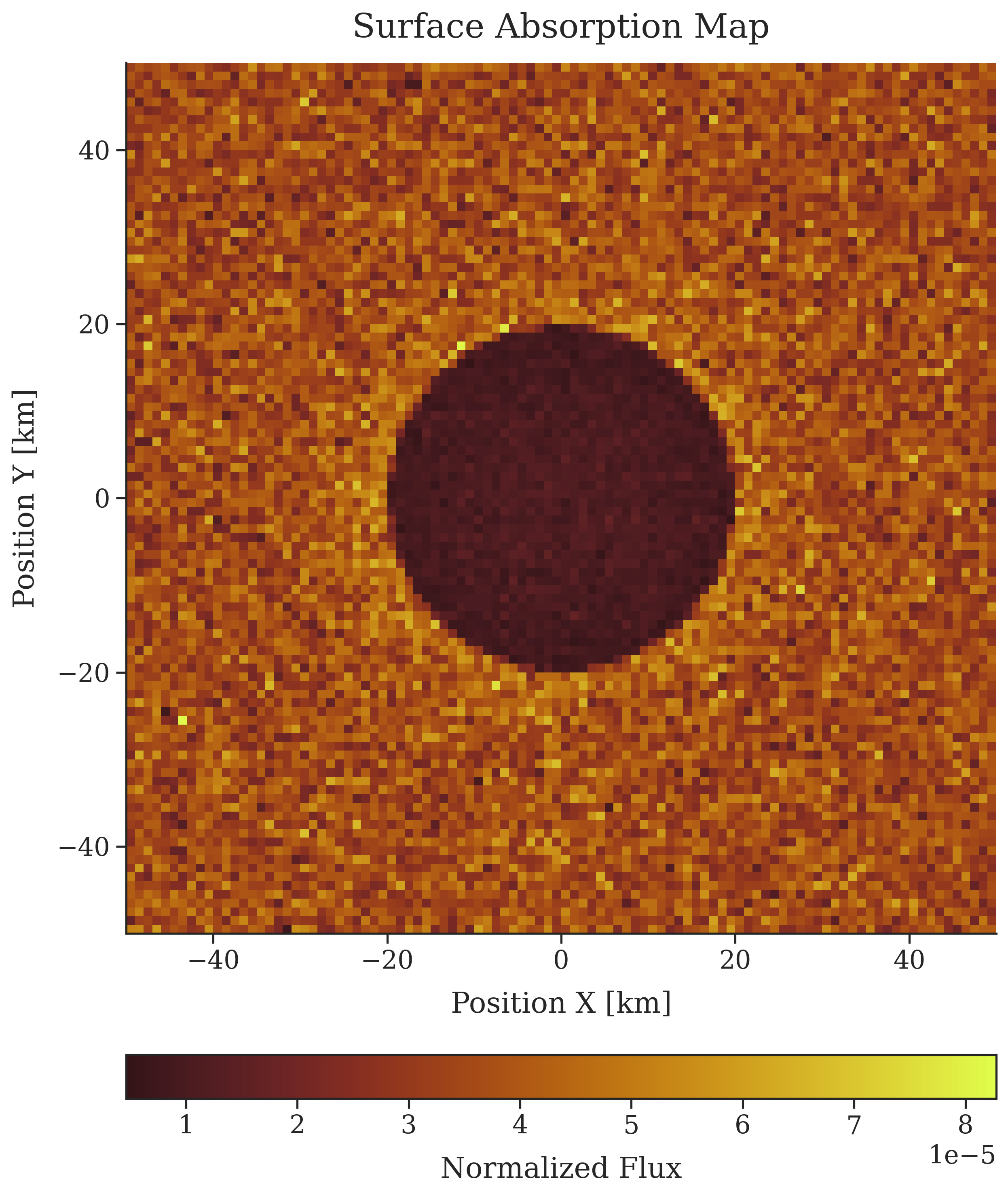
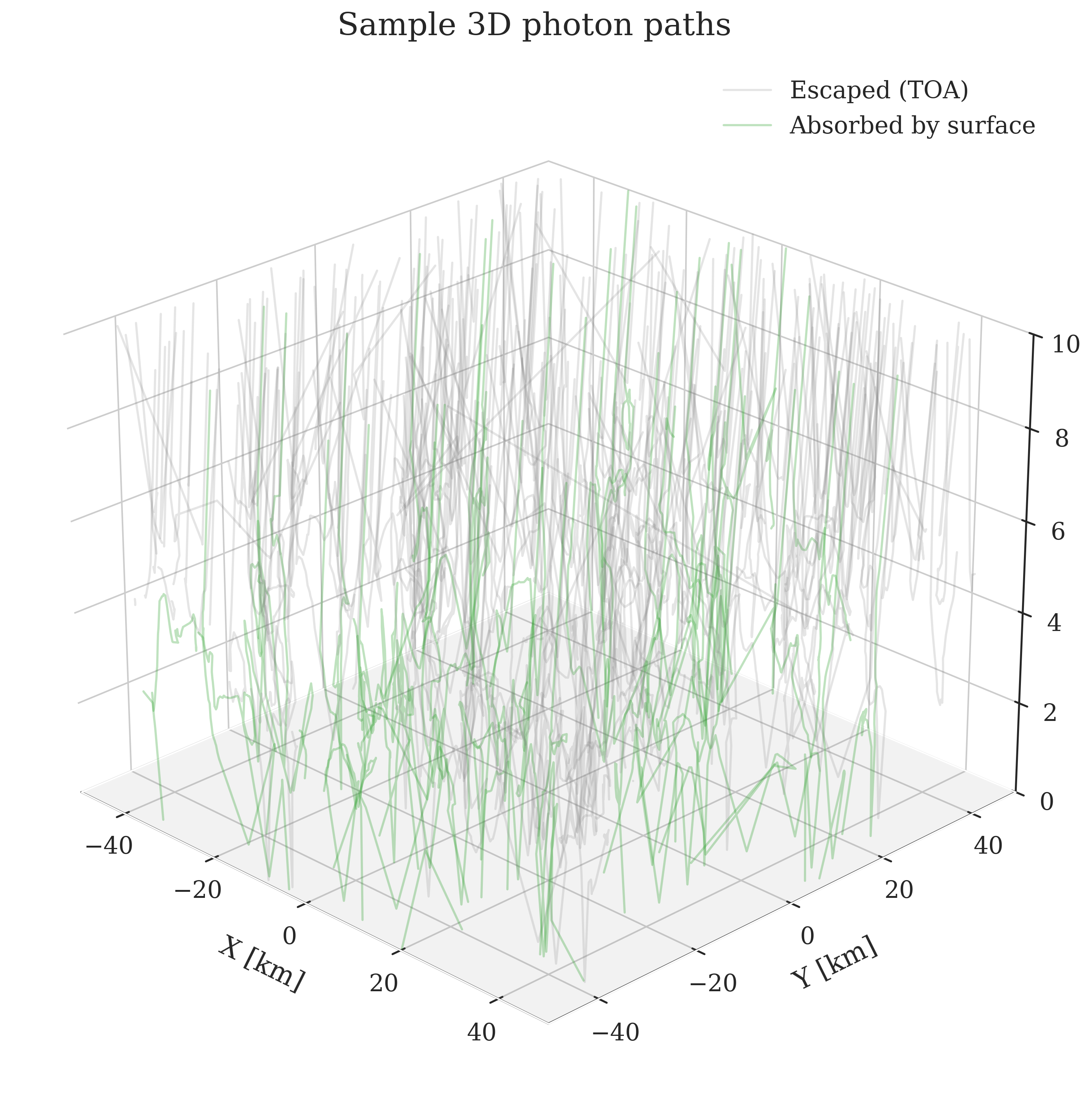
| 2D surface absorption map | Sample photon paths |
|---|---|
 |
 |
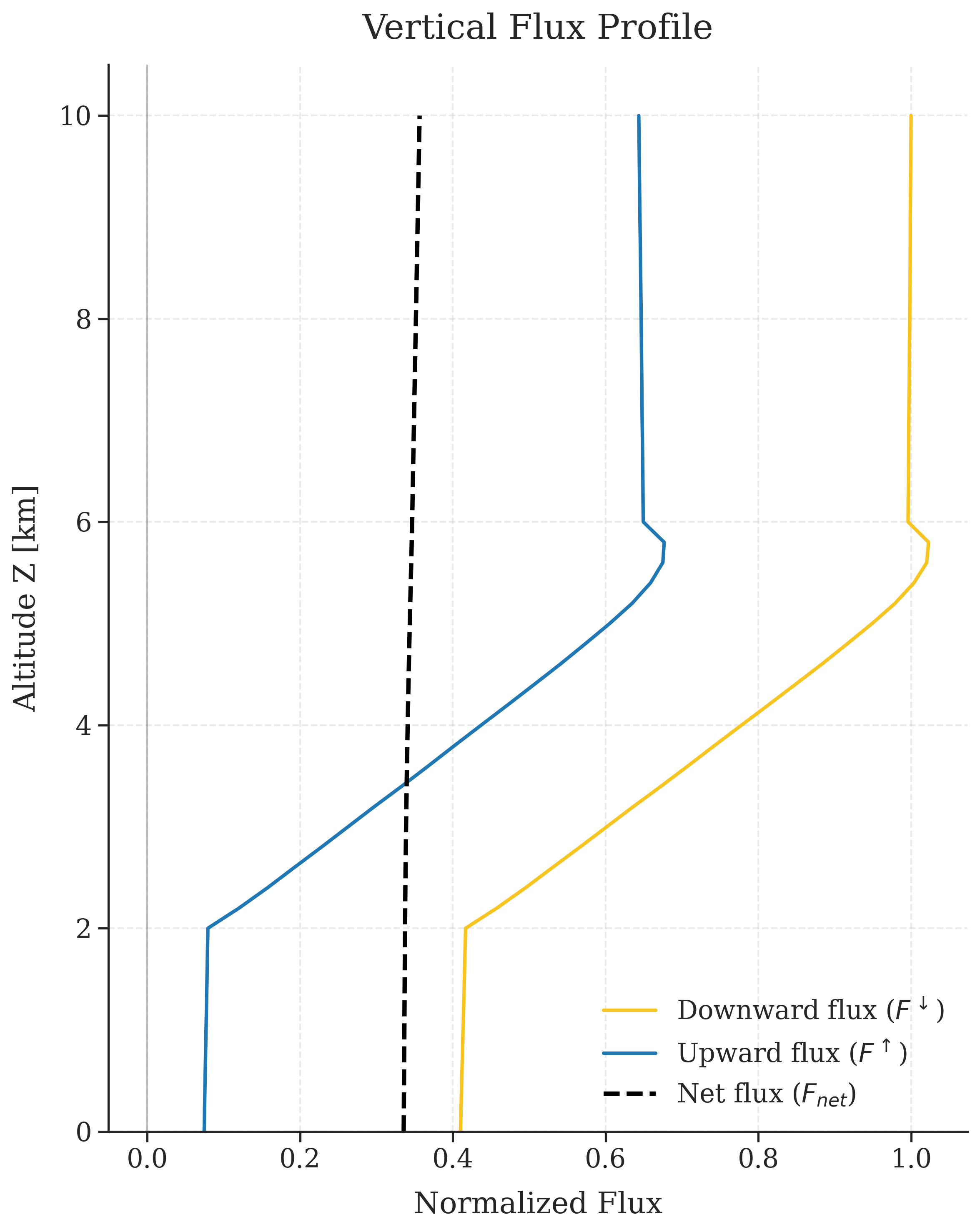
| Vertical flux profile | Vertical absorption profile |
 |
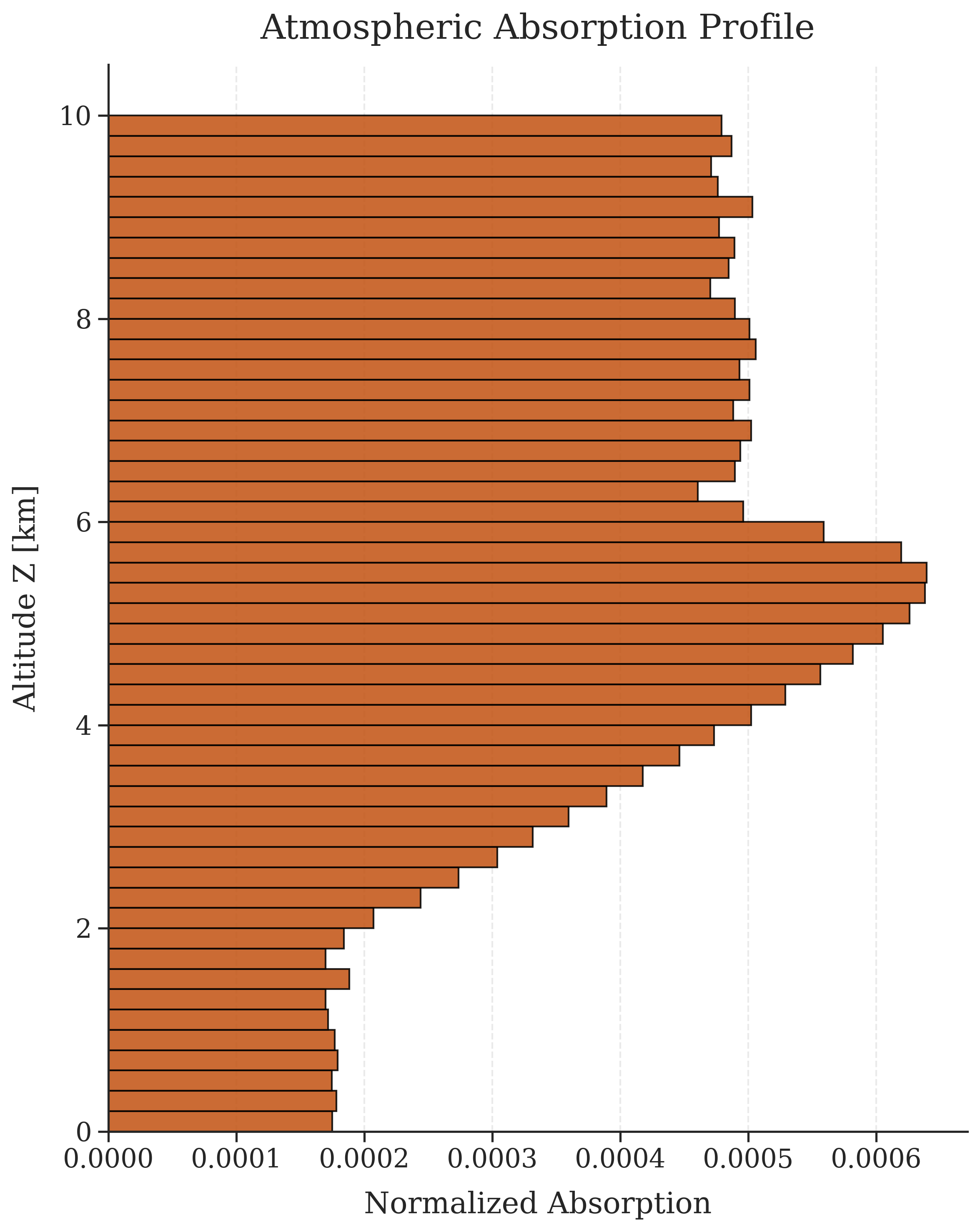 |
| Example outputs generated from the default configuration |
Overview
atmorad is a Monte Carlo radiative transfer model written in Python.
Monte Carlo handles multiple scattering and non-uniform geometry without solving the radiative transfer equation, which is often quite complex to do. The cost is poor performance in thick, weakly-absorbing atmospheres (e.g. clouds), where a photon scatters many times before it escapes or gets absorbed.
The code simulates photon transport through a plane-parallel atmosphere above a heterogeneous surface and records quantities such as radiative fluxes, absorption profiles, and surface energy deposition.
Motivation
I started it as a learning project during lectures on Radiative Processes in the Atmosphere at the Faculty of Physics, University of Warsaw.
The original goal was to better understand Monte Carlo radiative transfer by implementing the underlying algorithms from scratch.
It also became an opportunity to learn how to organize a github repository.
Current capabilities
- vectorized photon transport using NumPy arrays
- plane-parallel layered atmosphere (photons tracked in 3D)
- 2D surface maps, possibly heterogeneous
- Rayleigh and Henyey-Greenstein phase functions
- Lambertian and specular BRDFs
- xarray-compatible NetCDF/HDF5 output
- checkpointing and simulation resume
Current limitations
- monochromatic radiation
- no polarization
- plane-parallel atmosphere
- no validation against reference radiative transfer benchmarks yet
- atmospheric optical properties are currently wavelength-independent
Future work
- validation against standard radiative transfer models
- delta tracking for arbitrary 3D cloud geometries
- wavelength-dependent optical properties of materials
- roughness parameter in specular reflection and other BRDF models
- 3D surface topography
- spherical geometry for high zenith angles and whole-Earth simulations
Installation
Using uv (Recommended for project isolation, also works very fast):
> uv tool install atmorad
Using pip:
> pip install atmorad
Quickstart
CLI
Initialize a default configuration file in your current directory:
> atmorad --init
Run the simulation:
> atmorad simulation.toml
demo001/baseline: 100%|█████████████████████████████████████████████████████████| 400000/400000 [00:08<00:00, 48699.42 photons/s]

Simulation complete

experiment: demo001
scenario: baseline

runtime: 8.22 s
photons: 400_000

Energy distribution
------------------------------
toa escape               65.75%
surface absorption       34.23%
atmospheric absorption    0.03%
------------------------------

Result file:
  results/demo001/atmorad_demo001_baseline.nc
Check the results/ and plots/ directories for generated simulation artifacts and plots.
Python script
from atmorad import run

ds = run("simulation.toml")
Configuration
The simulation is controlled via a TOML configuration file. (click to expand)
# =============================================================================
# atmorad simulation configuration file
# =============================================================================

[metadata]
experiment_name = "demo001"
description     = "a demo simulation of radiative transfer over a heterogeneous surface."

[engine]
random_seed                   = 42
num_photons                   = 400_000
batch_size                    = 100_000  # photons per simulation chunk
roulette_weight_threshold     = 1e-4
roulette_survival_probability = 0.1      # 10% chance to survive with 10x multiplied weight
num_threads                   = 4
resume_from_checkpoint        = false

[source]
zenith_angle_deg  = 30
azimuth_angle_deg = 0
wavelength_nm     = 530  # only for reference, wavelength-dependent parameters not implemented yet

[domain]
size_x_km          = 100
size_y_km          = 100
boundary_condition = "periodic"

# -----------------------------------------------------------------------------
# active detectors (comment out a block to deactivate)
# -----------------------------------------------------------------------------

[detectors.energy_budget]

[detectors.trajectories]
max_tracked_paths = 200

[detectors.flux_profile]
vertical_resolution_km = 0.1

[detectors.absorption_profile]
vertical_resolution_km = 0.2

[detectors.flux_maps]
horizontal_resolution_km = 2.1
z_levels_km              = [0.0, 4.0, 10.0]

[detectors.surface_absorption_map]
horizontal_resolution_km = 2.1

[output]
save_plots = true
overwrite  = true
base_dir   = "results"
fig_dir    = "plots"

# -----------------------------------------------------------------------------
# material types and properties
# -----------------------------------------------------------------------------

[surface_materials.snow]
albedo = 0.85
brdf   = { type = "lambertian" }

[surface_materials.ocean]
albedo = 0.01
brdf   = { type = "specular", roughness = 0.0 }

[atmosphere_materials.air]
extinction_coeff_per_km = 0.01  # optical density
ssa                     = 0.999
phase_function          = { type = "rayleigh" }

[atmosphere_materials.light_clouds]
extinction_coeff_per_km = 1.0
ssa                     = 0.999999  # negligible absorption
phase_function          = { type = "hg", g = 0.85 }  # g > 0 means forward scattering

[atmosphere_materials.dark_clouds]
extinction_coeff_per_km = 5.0
ssa                     = 0.999999
phase_function          = { type = "hg", g = 0.85 }

# -----------------------------------------------------------------------------
# atmospheric layers (bottom to top)
# -----------------------------------------------------------------------------

[[layer]]
thickness_km = 2.0
components   = { air = 1.0 }

[[layer]]
thickness_km = 4.0
components   = { air = 1.0, dark_clouds = 0.9 }  # { material: extinction coefficient multiplier }

[[layer]]
thickness_km = 4.0
components   = { air = 1.0 }

# -----------------------------------------------------------------------------
# surface map configuration (choose one by uncommenting)
# -----------------------------------------------------------------------------

# [surface]
# type     = "uniform"
# material = "snow"

[surface]
type         = "circle"
radius_km    = 20.0
material_in  = "snow"
material_out = "ocean"

# [surface]
# type           = "split_half_x"
# material_left  = "snow"
# material_right = "ocean"

# [surface]
# type         = "checkerboard"
# tile_size_km = 10.0
# material_a   = "snow"
# material_b   = "ocean"

# -----------------------------------------------------------------------------
# scenarios and sweeps (batch experiments)
# -----------------------------------------------------------------------------

# scenario overrides: each block runs a separate simulation
# [[scenario]]
# name    = "checkerboard-surface"
# surface = { type = "checkerboard", tile_size_km = 10.0, material_a = "snow", material_b = "ocean" }

# [[scenario]]
# name               = "less-photons"
# engine.num_photons = 50_000
# engine.batch_size  = 12_500

# multiple sweep blocks are combined using a cartesian product
# [[sweep]]
# parameter = "source.zenith_angle_deg"
# values    = [0, 15, 30, 45, 60]

# [[sweep]]
# parameter = "source.azimuth_angle_deg"
# values    = [0, 45, 90, 135, 180]
Loading results
Results are stored as NetCDF4/HDF5 files and can be loaded directly with xarray: (click to expand)
import xarray as xr

# open NetCDF file
ds = xr.open_dataset("results/demo001/atmorad_demo001_baseline.nc", engine="h5netcdf")

# access arrays
map_2d = ds["surface_absorption_map"].values
flux_profile = ds["flux_down_profile"].values

# access scalars
total_reflected_energy = ds["energy_toa_outgoing"].item()
total_absorbed_surf = ds["energy_surface_absorbed"].item()

# access attributes
num_photons = ds.attrs["num_photons"]
sim_time = ds.attrs["simulation_time_s"]
active_detectors = ds.attrs["active_detectors"]
Or via atmorad:
from atmorad import load
ds = load("results/demo001/atmorad_demo001_baseline.nc")
Extracting configuration file from results
Each data .nc file contains configuration data used to run the simulation. You can extract it by running:
atmorad --extract-config <path-to-data.nc>
This creates an <exp_name>_<scen_name>_config.toml file in the current working directory.
Literature
- (in Polish) Script for lecture about Radiative Processes in the Atmosphere, Prof. K. Markowicz, Faculty of Physics, University of Warsaw, 2013.
Equations and algorithms
- L. G. Henyey, J. L. Greenstein, 1941, doi:10.1086/144246 — Henyey-Greenstein phase function.
- J. R. Frisvad, 2011, doi:10.1364/JOSAA.28.002436 — inverse sampling of the Rayleigh phase function.
- L. Wang, S. L. Jacques, L. Zheng, 1995, doi:10.1016/0169-2607(95)01640-F — rotation function and inverse sampling of Henyey-Greenstein phase function.
Acknowledgments
- I created this project inspired by the lectures on Radiative Processes in the Atmosphere by Prof. K. Markowicz, Faculty of Physics, University of Warsaw.
- I used an LLM as a programming aid during development.
Contributing
Contributions of any size are welcome. Open an issue to report a bug or to suggest something.
Release history Release notifications | RSS feed

Download files
Download the file for your platform. If you're not sure which to choose, learn more about installing packages.
Source Distribution
Built Distribution
Filter files by name, interpreter, ABI, and platform.
If you're not sure about the file name format, learn more about wheel file names.
Copy a direct link to the current filters
File details
Details for the file atmorad-0.3.0.tar.gz.
File metadata
- Download URL: atmorad-0.3.0.tar.gz
- Upload date:
- Size: 2.5 MB
- Tags: Source
- Uploaded using Trusted Publishing? No
- Uploaded via: uv/0.11.3 {"installer":{"name":"uv","version":"0.11.3","subcommand":["publish"]},"python":null,"implementation":{"name":null,"version":null},"distro":{"name":"Ubuntu","version":"24.04","id":"noble","libc":null},"system":{"name":null,"release":null},"cpu":null,"openssl_version":null,"setuptools_version":null,"rustc_version":null,"ci":null}
File hashes
| Algorithm | Hash digest | |
|---|---|---|
| SHA256 |
c10502857a96aa3719f984c400b159166778194b97eef5bbd9fa43b9bde27fb4
|
|
| MD5 |
3c5d500f0eb1602bc1ed314b3302f209
|
|
| BLAKE2b-256 |
af64f7b2ed23af4fa81bd93bc26c015e8a0771e989012516116f2ee9a460860b
|
File details
Details for the file atmorad-0.3.0-py3-none-any.whl.
File metadata
- Download URL: atmorad-0.3.0-py3-none-any.whl
- Upload date:
- Size: 44.2 kB
- Tags: Python 3
- Uploaded using Trusted Publishing? No
- Uploaded via: uv/0.11.3 {"installer":{"name":"uv","version":"0.11.3","subcommand":["publish"]},"python":null,"implementation":{"name":null,"version":null},"distro":{"name":"Ubuntu","version":"24.04","id":"noble","libc":null},"system":{"name":null,"release":null},"cpu":null,"openssl_version":null,"setuptools_version":null,"rustc_version":null,"ci":null}
File hashes
| Algorithm | Hash digest | |
|---|---|---|
| SHA256 |
19a2733d80640dbc63054091e4626e06640ba566f68e0d2f8170aea5e843c7b4
|
|
| MD5 |
4d0ac0bb76fd9726b14ac897de93e989
|
|
| BLAKE2b-256 |
b029ebf3cc95ebfe8dc49174d80dc5540a89ea5243227450c80bd21e3ed5ab9e
|






